Advanced Lane Finding

Detected Lane from Perspective View	Detected Lane from Birds-eye View

Overview

---

When we drive on the road, the lines on the road act as the references. To develope a self-driving car, one of the significant goals is to detect lane and automatically steer the vehicle.

In this project, the main goal is to build a pipeline to identify the lane boundaries in a video using cmputer vision techniques starting from camera caliaration to detect lane lines and calculate some characteristic of these lanes. The video project_video.mp4 is the video of the pipeline will work on in this project.

Goal

---

The goals / steps of this project are the following:

• Compute the camera calibration matrix and distortion coefficients given a set of chessboard images.
• Apply a distortion correction to the images (or videos).
• Use color transforms, gradients, etc., to create a thresholded binary image.
• Apply a perspective transform to rectify binary image ("birds-eye view").
• Detect lane pixels and fit to find the lane boundary.
• Determine the curvature of the lane and vehicle position with respect to center.
• Warp the detected lane boundaries back onto the original image.
• Output visual display of the lane boundaries and numerical estimation of lane curvature and vehicle position.

Files

---

The structure and useage of the files in this repository are as follows:

main_pipeline.ipynb: This part contains all the utility, visualization, preprocessing, computer vision techniques and vedio processing codes.

test_images: It contains 11 images extracted from the test videos.

test_videos: It contains 3 test videos: (1)project_video.mp4, (2)challenge_video.mp4, (3)harder_challenge_video.mp4

camera_cal: It contains chessboard images for clibration.

img: It stores the results during image processing.

utils: It contains the functions used for image processing in this project.

Pipeline

Camera Calibration

---

The OpenCV functions cv2.findChessboardCorners() and cv2.drawChessboardCorners() are used for image calibration. There are chessboard images stored in ./camera_cal/chessboard_6x8 and chessboard_6x9, taken from different angles with the same camera, and we'll use them as input for camera calibration routine.

The chessboard images have been used to calculate the camera calibration matrix and distortion coefficients, and these were used to remove distortion from one of the calibration images, demonstrating the effect.

cv2.findChessboardCorners() attempts to determine whether the input image is a view of the chessboard pattern and detect internal chessboard corners, and then cv2.drawChessboardCorners() will mark internal chessboard corners.

Arrays of object points, corresponding to the location of internal corners of a chessboard, and image points, the pixel locations of the internal chessboard corners determined by cv2.findChessboardCorners(), are fed to cv2.drawChessboardCorners() which returns camera calibration and distortion coefficients. The code are shown below:

gray = cv2.cvtColor(img,cv2.COLOR_BGR2GRAY)
ret, corners = cv2.findChessboardCorners(gray, (9,6), None)
if ret == True:
	marked_img = cv2.drawChessboardCorners(img, (9,6), corners, ret)

These will then be used by the OpenCV cv2.calibrateCamera() to find the camera calibration parameters from different views. These parameters will be fed to cv2.undistort function to correct for distortion on any image produced by the same camera. The code are shown below:

ret, mtx, dist, rvecs, tvecs = cv2.calibrateCamera(object_pts, image_pts, img_size, None, None)

The following figure shows the examples of distortion-corrected chessboard images.

Distortion Correction

---

The undistorted test image shows that distortion correction has been properly applied to images of highway driving. OpenCV provides cv2.undistort function, which transforms an image to compensate for radial and tangential lens distortion. The code are shown below:

undistort_img = cv2.undistort(img, mtx, dist, None, mtx)

The following figure shows the original view of the test images in `./test_images`

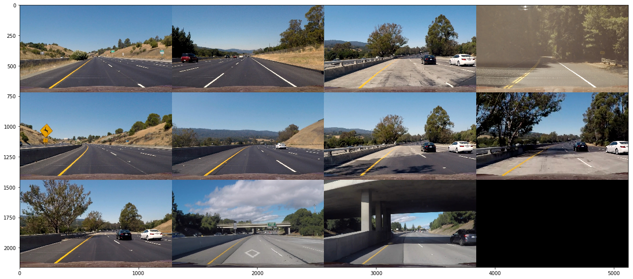
The following figure shows the undistorted test images

Perspective Transform

---

A common task in autonomous driving is to convert the vehicle’s camera view of the scene into a top-down "bird eye" view. We'll use OpenCV's cv2.getPerspectiveTransform and cv2.warpPerspective to do this task. First we need to define the region of interest for transformation. Next, we applied cv2.getPerspectiveTransform to calculate the transformation matrix. With the transformation matrix, we can easily get the image in bird-eye view The code are shown below:

src_region = np.float32([[(src_x1, src_y1), (src_x2, src_y2), (src_x3, src_x3), (src_x4, src_x4)]])
dst_region = np.float32([[(dst_x1, dst_y1), (dst_x2, dst_y2), (dst_x3, dst_x3), (dst_x4, dst_x4)]])

Mtx = cv2.getPerspectiveTransform(src_region, dst_region)
inv_Mtx = cv2.getPerspectiveTransform(dst_region, src_region)
birdeye_img = cv2.warpPerspective(img, Mtx, img_size, flags = cv2.INTER_LINEAR)      
perspective_img = cv2.warpPerspective(birdeye_img, inv_Mtx, img_size, flags = cv2.INTER_LINEAR)    

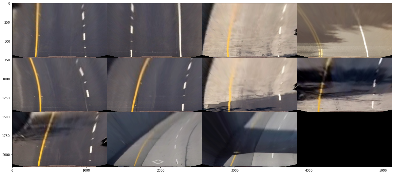
The following figure shows the test images after perspective transformation.

Contrast Enhancement

---

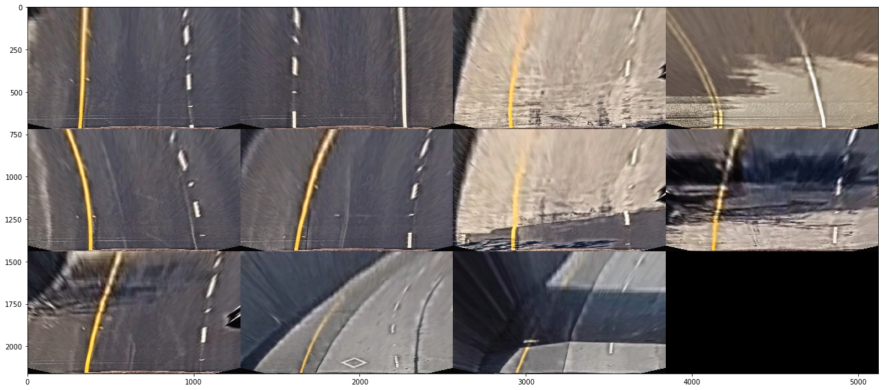
The edgue of the images are vague after perspective transform, so we tried to apply histogram equalization techniques to improve contrast in images. Histogram equalization computes several histograms, each corresponding to a distinct section of the image, and uses them to redistribute the lightness values of the image. It is therefore useful for improving the local contrast and enhancing the definitions of edges in each region of an image.

We converted image to LAB Color model and picked the image of L channel. To enhance the contrast, we applied cv2.createCLAHE and merge the CLAHE-enhanced L-channel with the a and b channel.

lab= cv2.cvtColor(img, cv2.COLOR_RGB2LAB)
l, a, b = cv2.split(lab)
clahe = cv2.createCLAHE(clipLimit=3.0, tileGridSize=(8,8))
cl = clahe.apply(l)
l_img = cv2.merge((cl,a,b))
Enhanced_img = cv2.cvtColor(l_img, cv2.COLOR_LAB2RGB)

The following figure shows the test images after applying contrast-limited adaptive histogram equalization.

Image Filters with Threshold

In this part, we will use color filter and Sobel operator to detect the lane lines in the image.

Threshold of Gradient, Gradient Magnitude and Gradient Direction

---

Applying the Sobel operator to an image is a way of taking the derivative of the image in the x or y direction. The operators for x, y can be defined cv2.Sobel

The magnitude of the gradient is the square root of the squares of the individual x and y gradients. It's important to note that the kernel size should be an odd number. The calculations of these three threshold are as follows:

gray = cv2.cvtColor(img, cv2.COLOR_RGB2GRAY)
sobelx = cv2.Sobel(gray, cv2.CV_64F, 1, 0)
sobely = cv2.Sobel(gray, cv2.CV_64F, 0, 1)
abs_sobelx = np.abs(sobelx)
abs_sobely = np.abs(sobely)

scaled_sobel = np.uint8(255*abs_sobelx/np.max(abs_sobelx)) # gradient

magnitude = np.sqrt(np.square(sobelx)+np.square(sobely))   # gradient magnitude
mag_scaled_sobel = np.uint8(255*magnitude/np.max(magnitude))  

dir_gradient = np.arctan2(abs_sobely, abs_sobelx) 		   # gradient direction
   
binary_filter = np.zeros_like(scaled_sobel)
binary_filter[(scaled_sobel >= grad_thresh[0]) & (scaled_sobel <= grad_thresh[1]) 
			& (mag_scaled_sobel >= mag_thresh[0]) & (mag_scaled_sobel <= mag_thresh[1])
			& (dir_gradient >= dir_thresh[0]) & (dir_gradient <= dir_thresh[1])] = 1

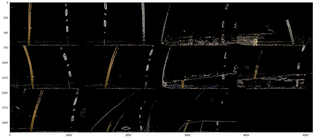
The following figure shows the test images filtered with threshold of Gradient ranged from 15 to 70.

The following figure shows the test images filtered with threshold of Gradient Magnitude ranged from 10 to 70.

The following figure shows the test images filtered with threshold of Gradient Direction ranged from 0.05 to 0.7 (radian).

Threshold of Color Space (HLS, HSV and RGB)

---

A color space is a specific organization of colors, which provide a way to categorize colors and filter specific colors. RGB is red-green-blue color space, HSV is hue-saturation-value color space, and HLS is hue-lightness-saturation color space. These are some of the most commonly used color spaces in image analysis. The uses of these color space are as follows, but we only take HLS as example because the precedure are the same.

hls_img = cv2.cvtColor(img, cv2.COLOR_RGB2HLS)
H_img = hls_img[:,:,0]
L_img = hls_img[:,:,1]
S_img = hls_img[:,:,2]

H_binary = np.zeros_like(H_img)
H_binary[(H_img > H_thresh[0]) & (H_img <= H_thresh[1])] = 1

L_binary = np.zeros_like(L_img)
L_binary[(L_img > L_thresh[0]) & (L_img <= L_thresh[1])] = 1

S_binary = np.zeros_like(S_img)
S_binary[(S_img > S_thresh[0]) & (S_img <= S_thresh[1])] = 1

combined_binary = np.zeros_like(img[:,:,0])
combined_binary[(H_binary == 1) | (L_binary == 1) | (S_binary == 1)] = 1

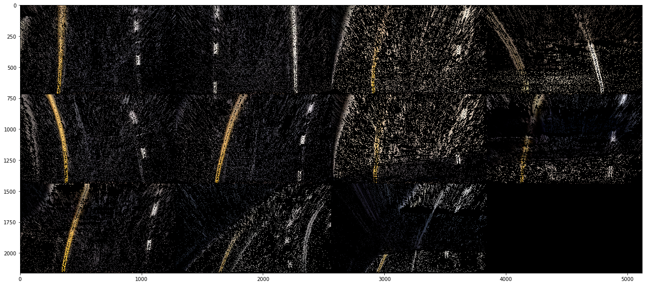
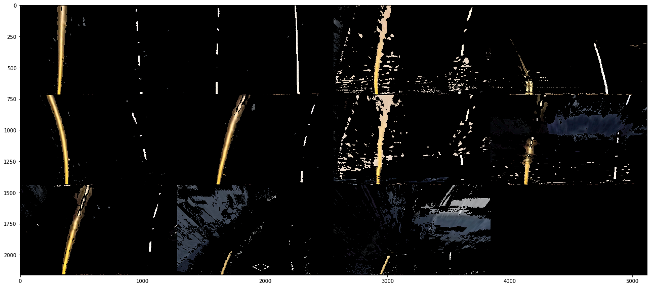
The following figure shows the test images filtered with threshold of HLS.

The following figure shows the test images filtered with threshold of HSV.

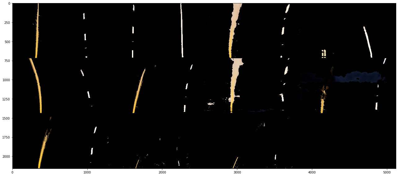
The following figure shows the test images filtered with threshold of RGB.

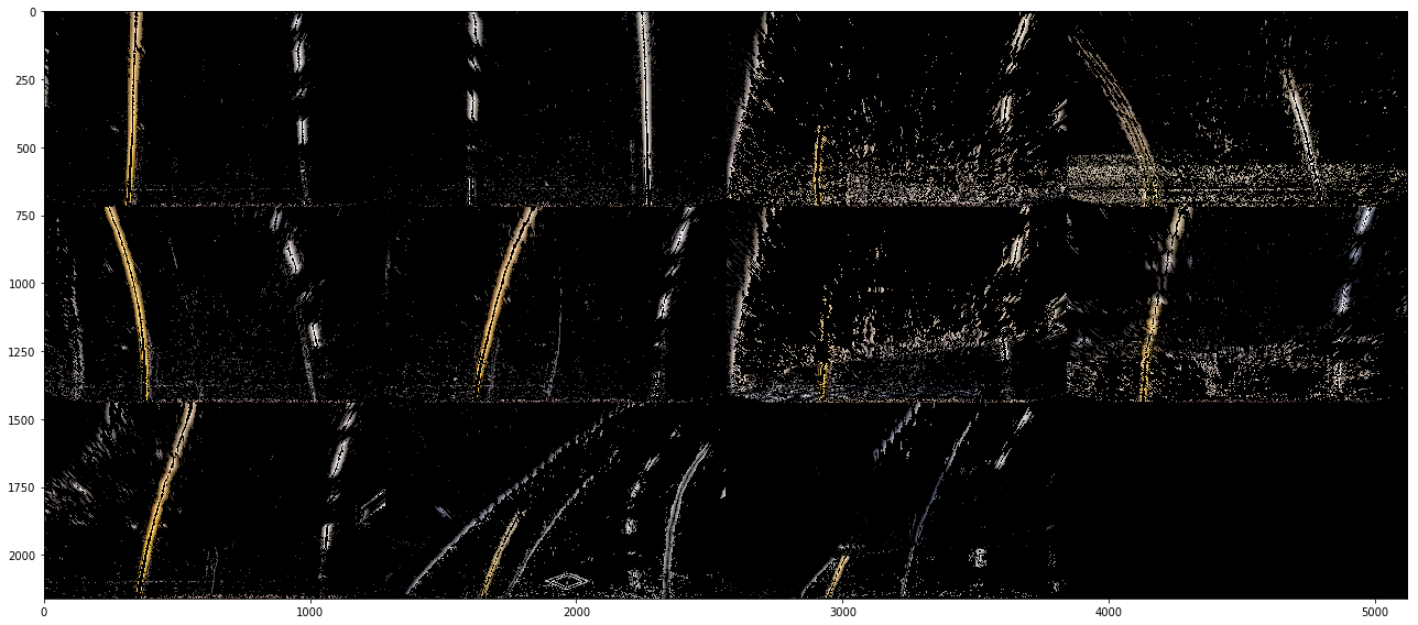
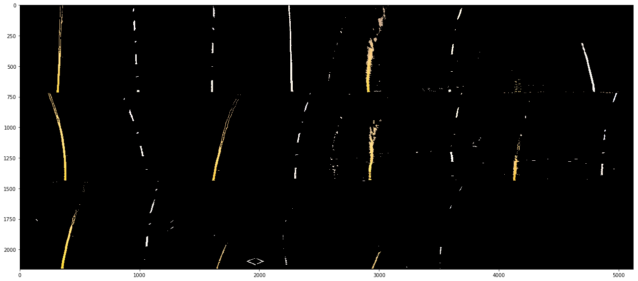
The following figure overviews the result of test images after applying each filter.

Lane Line Identification with Sliding Window

---

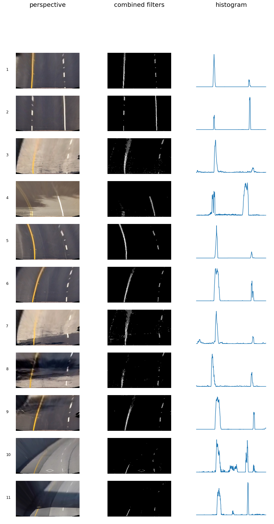
After applying calibration, perspective transform and thresholding to a road image, we get a binary image where the lane lines stand out clearly. Next, we take a histogram along all the columns in the lower half of a image to decide which part belongs to the left line and which part belongs to the right line.

The following figure shows the result of test images after applying peak detection.

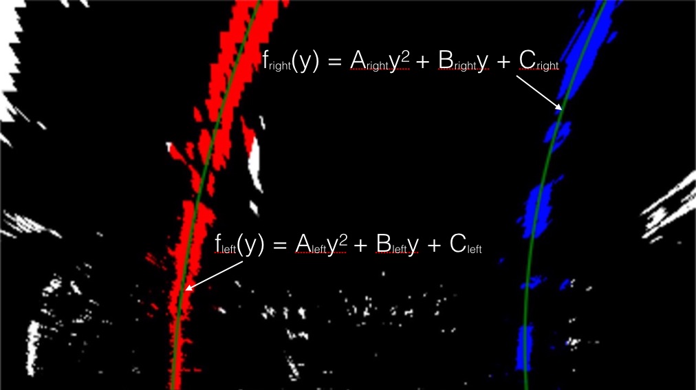
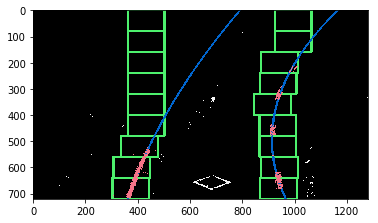
In the thresholded image, pixels are either 0 or a number larger than 0, so the two most prominent peaks in this histogram will be good indicators of the x-position of the base of the lane lines. We can use that as a starting point for where to search for the lines together with the sliding window, placed around the line centers, to find the lines up to the top of the frame. With the identified lane-line pixels, we applied numpy.polyfit(x,y,2) to fit their positions with a second order polynomial.

The following figure show an example of pixels falling in the region of window.

The following figure shows an example of lane line detection with sliding window.

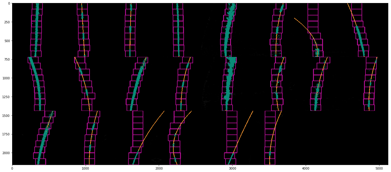
The following figure shows the detected lane lines of the test images with sliding window.

Calculation of the Lane Curvature and the Position of the Vehicle with respect to center.

---

To steer the vehicle, we calculated the lane curvature and converted the result from pixels to real world measurements. The radius of curvature may be given in meters assuming the curve of the road follows a circle. For the position of the vehicle, we assume the camera is mounted at the center of the car, and the deviation of the midpoint of the lane from the center of the image is the offset we look for.

With the data from authority, the images with U.S. regulations that require a minimum lane width of 12 feet or 3.7 meters, and the dashed lane lines are 10 feet or 3 meters long each. The codes of calculation are as follows:

# Define y-value where we calculate radius of curvature, we choose the position of vehicle which is the bottom of the image.
y = image.shape[0]

# Define conversions in x and y from pixels space to meters
ym_per_pix = 30/720 # meters per pixel in y dimension
xm_per_pix = 3.7/700 # meters per pixel in x dimension

# Fit new polynomials to x,y in world space
left_fit_cr = np.polyfit(y * ym_per_pix, leftx * xm_per_pix, 2)
right_fit_cr = np.polyfit(y * ym_per_pix, rightx * xm_per_pix, 2)

# Calculate the radii of curvature in meters
left_curverad = ((1 + (2*left_fit_cr[0]*y_eval*ym_per_pix + left_fit_cr[1])**2)**1.5) / np.absolute(2*left_fit_cr[0])
right_curverad = ((1 + (2*right_fit_cr[0]*y_eval*ym_per_pix + right_fit_cr[1])**2)**1.5) / np.absolute(2*right_fit_cr[0])

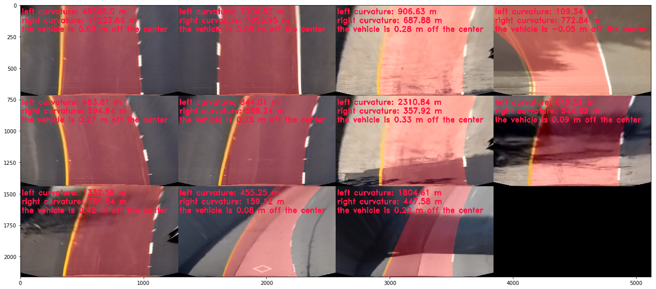
The following figure shows the test images with lane curvature, deviation from road center, detected region between lanes from bird-eye view.

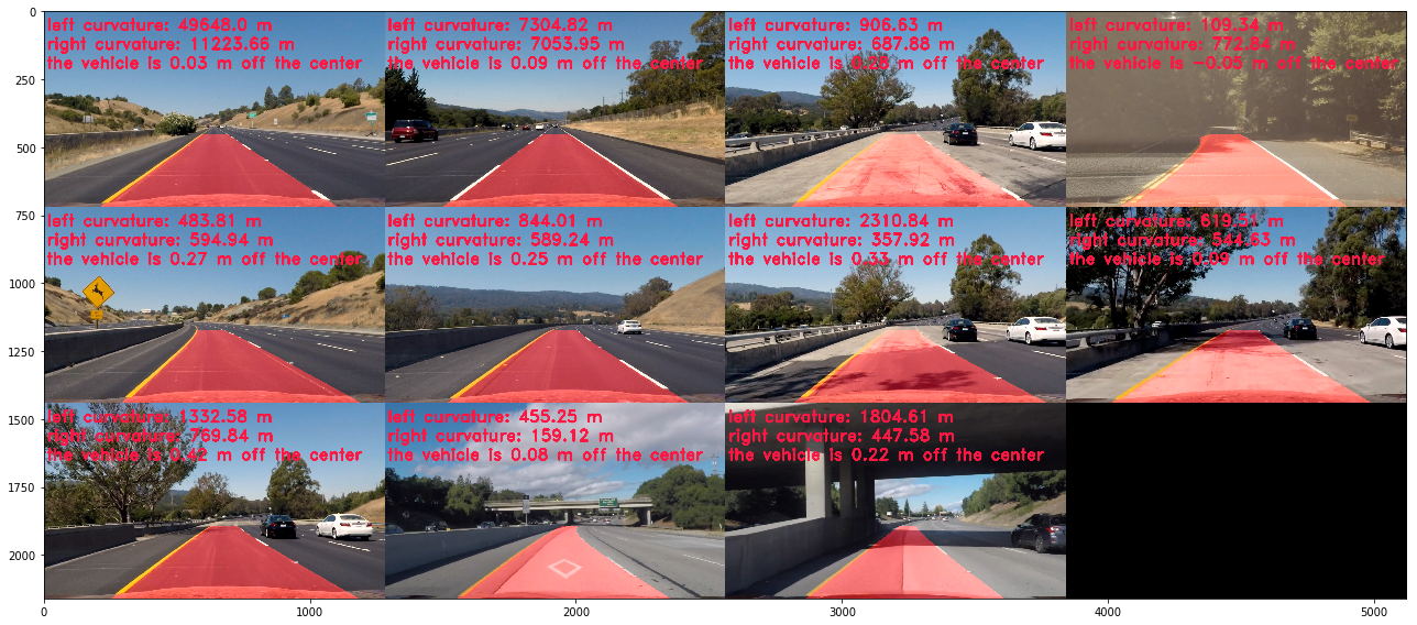
The following figure shows the test images with lane curvature, deviation from road center, detected region between lanes from perspective view.

Result

---

1. The pipeline works well on the project.ma4 which of result could be found in bird view and perspective view, but performs terribly in challenge_video.mp4 and harder_challenge.mp4. The reasons are mainly from the noises such as edge of the road shoulder, fence, shadow, sunshine, stains, road segment with different colors due to respilled asphalt. I applied combination of thresholding techniques and add up detected pixels. I give more weights to the pixels with high values because it was detected as a lane more times than other pixels, but the results were still insatisfiable. One thing I also have seen is that the L channel from LUV with lower and upper thresholds around 225 & 255 respectively works very well to pick out the white lines, even in the parts of the video with heavy shadows and brighter pavement. Another one is the B channel from LAB which does a great job with the yellow lines with thresholds around 155 & 200.

2. The lane line on the far side is unclear. I applied contrast enhancement techniques under LAB color space, but the performance did not change much. Actually, these techniques were applied to images from bird view, which are quite vague after transforming. One approach could be using thresholds on perspective images whose lanes are still clear. In addition, Canny edge detection and Hough line detection were not applied in this pipeline, but they actually can assist in enhancing the outline of lane line. All in all, the lane lines after the perspective transform appear very close to parallel in the birds-eye view images for project video.

3. Some lanes are dash lines. Instead, the lines at the road shoulder are solid lines. The maginitude of dash line in histogram is less than that of solid line. I tried to give more weight to color filters, but the color filter cannot resist the noise of shadow due to the change of color. Another issue is the gap between dash lines could be quite large. In this case, the height of the window should be larger to prevent the low peak in histogram.

Conclusion

---

1. The pipeline detects the lane line from scratch for each frame. It will work well in simple situation like project.ma4. However, the sliding window might lose the real lane due to the bad window size and terrible initial state such as sunshine which made the lane line disapear in the frame. Some caches could be imported to memorize the previous fitting lane to assist the guess of lane line.

2. Sometimes the sliding window can not find any lane pixels. Except the dash line, there are two common cases: dash line and lane with low curvature radii. For these two cases, the window needs to be long and wide enough, but large window might detect noises which influces fitting line.

   • One solution is to reuse the binary filters when the sliding window could not find lane pixels.
   • The second solution is to move the window based on the detected pixels with low y values which helps sliding window catch up the fast-changing lane with low curvature radii.
   • The third solution could be interpolting from the noises. Sometimes there are detected lines from the fence, road shoulder, etc. I took them as noises in the pipeline, but it could be used to guess the lane shape and direction with Canny edge detection. Once we got the information of other egde, the orientation of current lane and road condition could be understood better. Furthurmore, we can make decisions such as changing the lane.

3. After finding a confident detection in one frame, the histogram search could be skipped in the next frame and go straight with the search in a tight proximity around the polynomials from the previous frames. An example of how to implement it is as follows: I recommend implementing something like this:

if line was detected in previous frame:
  skip sliding windows
else:
  sliding window search

4. Even when everything is working, the detected lines could jump around from frame to frame a bit and it can be preferable to smooth over the last n frames of video to obtain a cleaner result. One thing to be careful with here is that the lane should be shifted horizontally after applying the perspective transform, otherwise there can be issues with calculating the vehicle offset from center because the camera position will no longer be located at the center of the image.

Possible improvement

---

1. To get accurate estimates of the measurements (where the lane lines are, estimation of how much the road is curved and where the vehicle is located with respect to the center of the lane. It is important to make sure that appropriate pixel-to-meter conversion factors is used based on the perspective transform applied to the images. For example, a conversion of xm_per_pix = 3.7/700 assumes that the lane is 700 pixels wide in the warped images, so if the actual lane width differs from 700 pixels you should replace the 700 with the actual width of the lane.

2. Other improvements could be the implementation of some sanity checks which look for unreasonable detections to prevent them being used in the output video. For sanity checks, some of the following criteria could be considered:

• Are the two polynomials an appropriate distance apart based on the known width of a highway lane?
• Do the two polynomials have same or similar curvature?
• Have these detections deviated significantly from those in recent frames?

When a sanity check fails in a single frame, instead of displaying the lines that with errors, the current detection could be discarded and reuse the confident detections from prior frames.

Reference

---

• U.S. Road Regulation
• Curvature formula

Appendix

---

1. The detail of code for searching without sliding windows is as follows:

# Assume you now have a new warped binary image 
# from the next frame of video (also called "binary_warped")
# It's now much easier to find line pixels!
nonzero = binary_warped.nonzero()
nonzeroy = np.array(nonzero[0])
nonzerox = np.array(nonzero[1])
margin = 100
left_lane_inds = ((nonzerox > (left_fit[0]*(nonzeroy**2) + left_fit[1]*nonzeroy + 
left_fit[2] - margin)) & (nonzerox < (left_fit[0]*(nonzeroy**2) + 
left_fit[1]*nonzeroy + left_fit[2] + margin))) 

right_lane_inds = ((nonzerox > (right_fit[0]*(nonzeroy**2) + right_fit[1]*nonzeroy + 
right_fit[2] - margin)) & (nonzerox < (right_fit[0]*(nonzeroy**2) + 
right_fit[1]*nonzeroy + right_fit[2] + margin)))  

# Again, extract left and right line pixel positions
leftx = nonzerox[left_lane_inds]
lefty = nonzeroy[left_lane_inds] 
rightx = nonzerox[right_lane_inds]
righty = nonzeroy[right_lane_inds]
# Fit a second order polynomial to each
left_fit = np.polyfit(lefty, leftx, 2)
right_fit = np.polyfit(righty, rightx, 2)
# Generate x and y values for plotting
ploty = np.linspace(0, binary_warped.shape[0]-1, binary_warped.shape[0] )
left_fitx = left_fit[0]*ploty**2 + left_fit[1]*ploty + left_fit[2]
right_fitx = right_fit[0]*ploty**2 + right_fit[1]*ploty + right_fit[2]

2. visualize the detected lane

# Create an image to draw on and an image to show the selection window
out_img = np.dstack((binary_warped, binary_warped, binary_warped))*255
window_img = np.zeros_like(out_img)
# Color in left and right line pixels
out_img[nonzeroy[left_lane_inds], nonzerox[left_lane_inds]] = [255, 0, 0]
out_img[nonzeroy[right_lane_inds], nonzerox[right_lane_inds]] = [0, 0, 255]

# Generate a polygon to illustrate the search window area
# And recast the x and y points into usable format for cv2.fillPoly()
left_line_window1 = np.array([np.transpose(np.vstack([left_fitx-margin, ploty]))])
left_line_window2 = np.array([np.flipud(np.transpose(np.vstack([left_fitx+margin, 
                              ploty])))])
left_line_pts = np.hstack((left_line_window1, left_line_window2))
right_line_window1 = np.array([np.transpose(np.vstack([right_fitx-margin, ploty]))])
right_line_window2 = np.array([np.flipud(np.transpose(np.vstack([right_fitx+margin, 
                              ploty])))])
right_line_pts = np.hstack((right_line_window1, right_line_window2))

# Draw the lane onto the warped blank image
cv2.fillPoly(window_img, np.int_([left_line_pts]), (0,255, 0))
cv2.fillPoly(window_img, np.int_([right_line_pts]), (0,255, 0))
result = cv2.addWeighted(out_img, 1, window_img, 0.3, 0)
plt.imshow(result)
plt.plot(left_fitx, ploty, color='yellow')
plt.plot(right_fitx, ploty, color='yellow')
plt.xlim(0, 1280)
plt.ylim(720, 0)