| marp |
|---|
true |
- Discover the general architecture of convolutional neural networks.
- Understand why they perform better than plain neural networks for image-related tasks.
The visual world has the following properties:
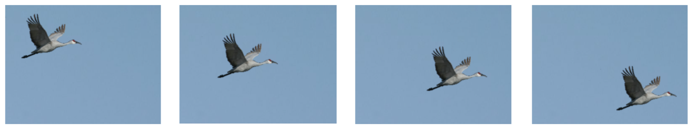
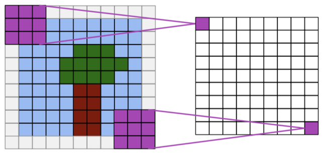
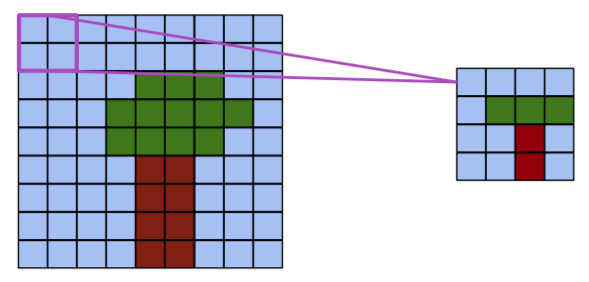
- Translation invariance.
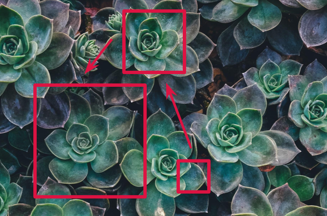
- Locality: nearby pixels are more strongly correlated
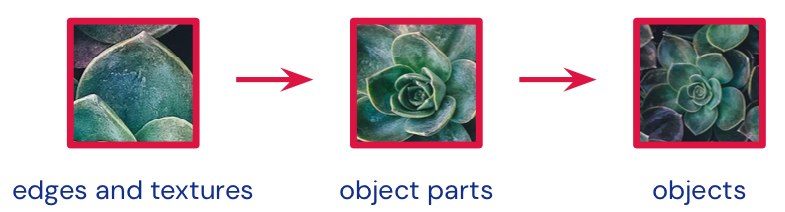
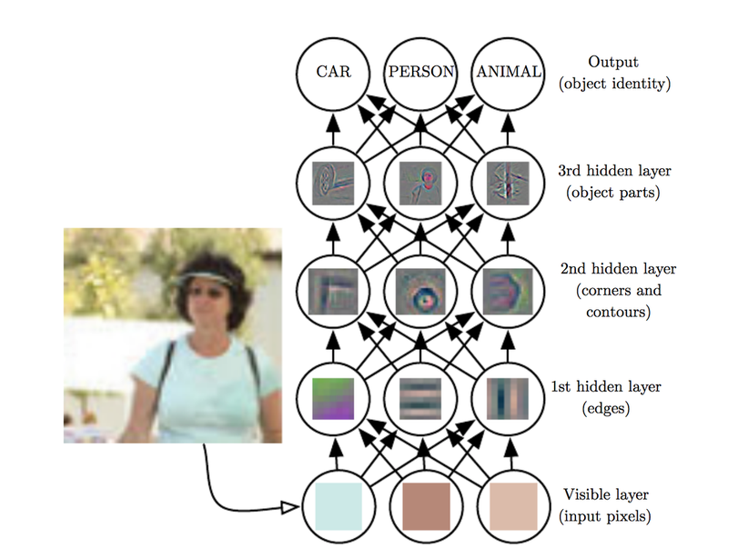
- Spatial hierarchy: complex and abstract concepts are composed from simple, local elements.
Classical models are not designed to detect local patterns in images.
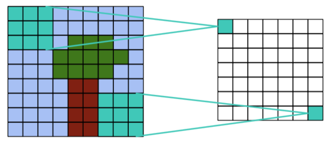
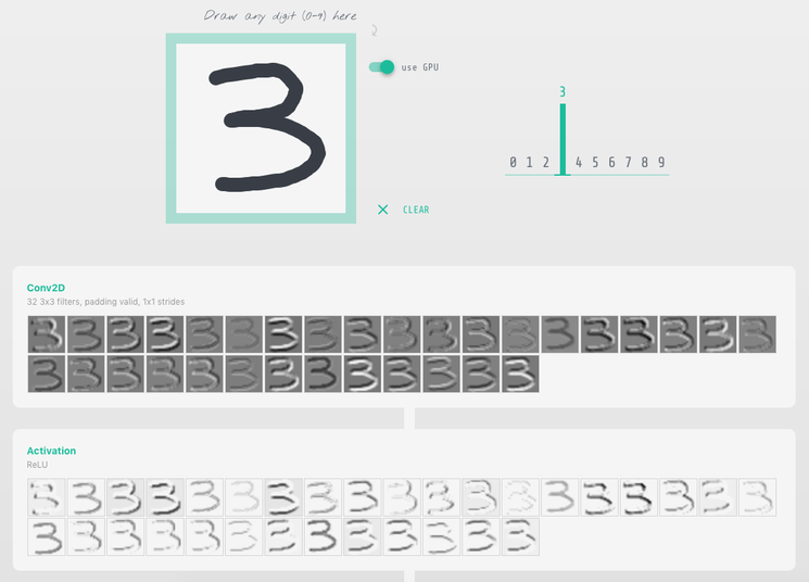
Apply a kernel to data. Result is called a feature map.

- Filter dimensions: 2D for images.
- Filter size: generally 3x3 or 5x5.
- Number of filters: determine the number of feature maps created by the convolution operation.
- Stride: step for sliding the convolution window. Generally equal to 1.
- Padding: blank rows/columns with all-zero values added on sides of the input feature map.
Output size = input size - kernel size + 1
Output size = input size + kernel size - 1
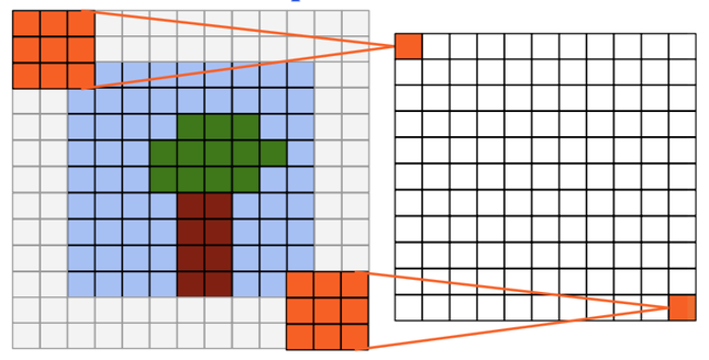
Output size = input size
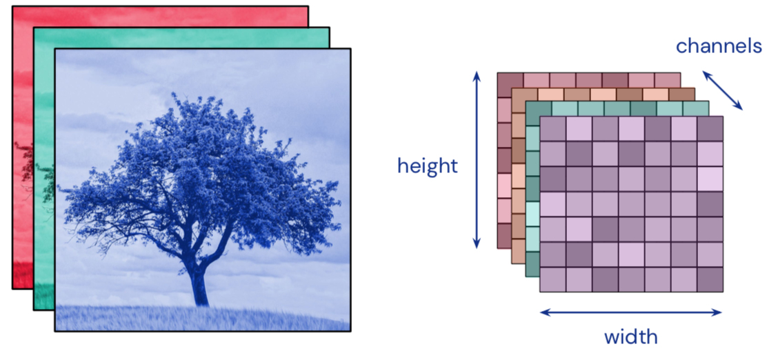
- Convolution input data is 3-dimensional: images with height, width and color channels, or features maps produced by previous layers.
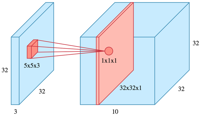
- Each convolution filter is a collection of kernels with distinct weights, one for every input channel.
- At each location, every input channel is convolved with the corresponding kernel. The results are summed to compute the (scalar) filter output for the location.
- Sliding one filter over the input data produces a 2D output feature map.

- Applied to the (scalar) convolution result.
- Introduces non-linearity in the model.
- Standard choice: ReLU.
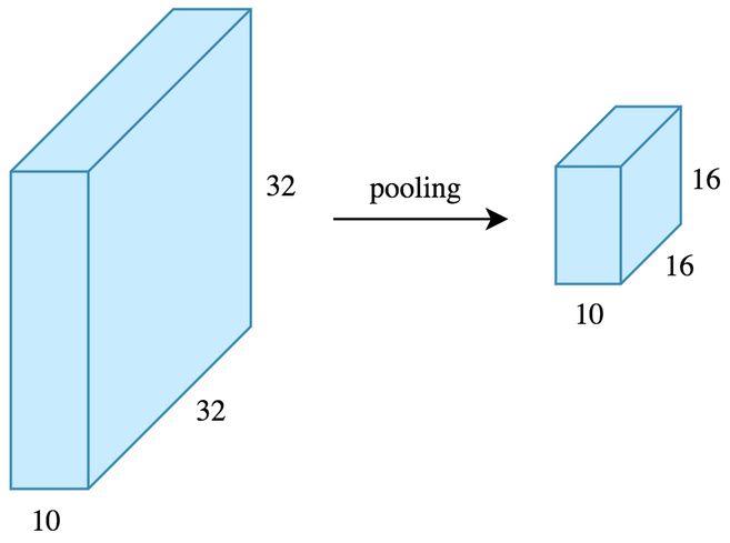
- Reduces the dimensionality of feature maps.
- Often done by selecting maximum values (max pooling).
Same principle as a dense neural network: backpropagation + gradient descent.
For convolution layers, the learned parameters are the values of the different kernels.
Backpropagation In Convolutional Neural Networks
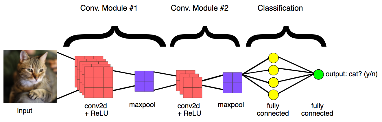
- Convolution layers act as feature extractors.
- Dense layers use the extracted features to classify data.


- ImageNet Large Scale Visual Recognition Challenge
- Worldwide image classification challenge based on the ImageNet dataset.

Trained on 2 GPU for 5 to 6 days.


- 9 Inception modules, more than 100 layers.
- Trained on several GPU for about a week.

- 152 layers, trained on 8 GPU for 2 to 3 weeks.
- Smaller error rate than a average human.


-
Challenges
- Computational complexity
- Optimization difficulties
-
Solutions
- Careful initialization
- Sophisticated optimizers
- Normalisation layers
- Network design
A pretrained convnet is a saved network that was previously trained on a large dataset (typically on a large-scale image classification task). If the training set was general enough, it can act as a generic model and its learned features can be useful for many problems.
It is an example of transfer learning.
There are two ways to use a pretrained model: feature extraction and fine-tuning.
Reuse the convolution base of a pretrained model, and add a custom classifier trained from scratch on top ot if.
State-of-the-art models (VGG, ResNet, Inception...) are regularly published by top AI institutions.
Slightly adjusts the top feature extraction layers of the model being reused, in order to make it more relevant for the new context.
These top layers and the custom classification layers on top of them are jointly trained.
