| marp | math |
|---|---|
true |
true |
- Discover the terminology and core concepts of supervised learning.
- Understand how a supervised ML system can be formalized.
- Some data to learn from.
- A model to transform data into results.
- A loss function to quantify how well (or badly) the model is doing.
- An optimization algorithm to update the model according to the loss function.
A feature is an attribute (property) of the data given to the model: the number of rooms in a house, the color of a pixel in an image, the presence of a specific word in a text, etc. Most of the time, they come under numerical form.
A simple ML project might use a single feature, while more sophisticated ones could use millions of them.
They are often denoted using the
A label (or class in the context of classification), is a result the model is trying to predict: the future price of an asset, the nature of the animal shown in a picture, the presence or absence of a face, etc.
They are often denoted using the
An sample, also called an example, is a particular instance of data: an individual email, an image, etc.
A labeled sample includes both its feature(s) and the associated label(s) to predict. An unlabeled sample includes only feature(s).
Inputs correspond to all features for one sample of the dataset.
They are often denoted using the
-
$m$ : number of samples in the dataset. -
$n$ : number of features for one sample. -
$\pmb{x}^{(i)}, i \in [1,m]$ : vector of$n$ features. -
$x^{(i)}_j, j \in [1,n]$ : value of the $j$th feature for the $i$th data sample.
Targets are the expected results (labels) associated to a data sample, often called the ground truth. They are often denoted using the
Some ML models have to predict more than one value for each sample (for example, in multiclass classification). In that case,
-
$K$ : number of labels associated to a data sample. -
$\pmb{y}^{(i)}, i \in [1,m]$ : expected results for the $i$th sample. -
$y^{(i)}_k, k \in [1,K]$ : actual value of the $k$th label for the $i$th sample.
Many ML models expect their inputs to come under the form of a
Accordingly, expected results are often stored in a
The core data structure of Machine Learning, a tensor is a multidimensional array of primitive values sharing the same type (most often numerical). For example, inputs and target matrices are stored as tensors in program memory.
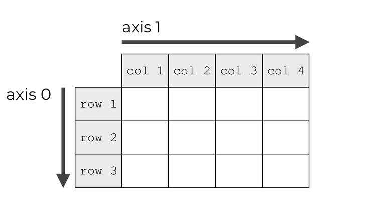
- A tensor’s dimension is also called an axis.
- A tensor’s rank is its number of axes.
- A tensor’s shape describes the number of values along each axis.
A scalar is a rank 0 (0D) tensor, a vector is a rank 1 (1D) tensor and a matrix is a rank 2 (2D) tensor.
Many tensor operations can be applied along one or several axes. They are indexed starting at 0.
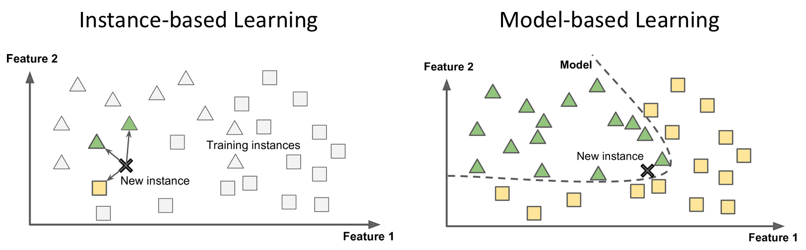
The representation learnt from data during training is called a model. It defines the relationship between features and labels.
Most (but not all) ML systems are model-based.
- Training: using labeled samples, the model learns to find a relationship between features and labels.
- Inference: the trained model is used to make predictions on unlabeled samples (new data unseen during training).
Parameters, sometimes called weights, are the internal values that affect the computed output of a model. During the training phase, they are algorithmically adjusted for optimal performance w.r.t the loss function. The set of parameters for a model is often denoted
They are not to be confused with hyperparameters, which are configuration properties that constrain the model: the maximum depth of a decision tree, the number of layers in a neural networks, etc. Hyperparameters are statically defined before training by the user or by a dedicated tool.
Mathematically speaking, a model is a function of the inputs that depends on its parameters and computes results (which will be compared to targets during the training process).
This function, called the hypothesis function, is denoted
$$\pmb{y'}^{(i)} = \begin{pmatrix} \ y'^{(i)}_1 \ \ y'^{(i)}_2 \ \ \vdots \ \ y'^{(i)}K \end{pmatrix} = h{\pmb{\omega}}(\pmb{x}^{(i)}) \in \mathbb{R}^K$$
-
$\pmb{y'}^{(i)}, i \in [1,m]$ : model prediction for the $i$th sample. -
$y'^{(i)}_k, k \in [1,K]$ : predicted output for the $k$th label of the $i$th sample.
Model predictions for the whole dataset can be stored in a
$$\pmb{Y'} = \begin{bmatrix} \ \pmb{y'}^{(1)T} \ \ \pmb{y'}^{(2)T} \ \ \vdots \ \ \pmb{y'}^{(m)T} \ \end{bmatrix} = \begin{bmatrix} \ y'^{(1)}_1 & y'^{(1)}_2 & \cdots & y'^{(1)}_K \ \ y'^{(2)}_1 & y'^{(2)}_2 & \cdots & y'^{(2)}_K \ \ \vdots & \vdots & \ddots & \vdots \ \ y'^{(m)}_1 & y'^{(m)}_2 & \cdots & y'^{(m)}K \end{bmatrix} = h{\pmb{\omega}}(\pmb{X}) \in \mathbb{R}^{m \times K}$$
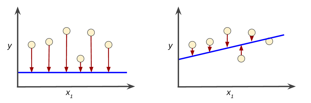
The loss function, also called cost function or objective function, quantifies the difference, often called error, between targets (expected results) and actual results computed by the model. Its value at any given time is a scalar called the loss value, or simply loss.
By convention, loss functions are usually defined so that lower is better, hence their name. If the model's prediction is perfect, the loss value is zero.
The loss function is generally denoted
Mathematically, it depends on the inputs
$\pmb{X}$ , the expected results$\pmb{Y}$ and the model parameters$\pmb{\omega}$ . However, during model training,$\pmb{X}$ and$\pmb{Y}$ can be treated as constants. Thus, the loss function depends solely on$\pmb{\omega}$ and will be denoted$\mathcal{L(\pmb{\omega})}$ .
The choice of the loss function depends on the problem type.
For regression tasks, a popular choice is the Mean Squared Error a.k.a. squared L2 norm.
$$\mathcal{L}{\mathrm{MSE}}(\pmb{\omega}) = \frac{1}{m}\sum{i=1}^m (h_{\pmb{\omega}}(\pmb{x}^{(i)}) - \pmb{y}^{(i)})^2 = \frac{1}{m}{{\lVert{h_{\pmb{\omega}}(\pmb{X}) - \pmb{Y}}\rVert}_2}^2$$
Used only during the training phase, it aims at finding the set of model parameters (denoted $\pmb{\omega^}$ or $\pmb{\theta^}$) that minimizes the loss value.
Depending on the task and the model type, several algorithms of various complexity exist.