Antialiased CNNs [Project Page] [Paper] [Talk]

Making Convolutional Networks Shift-Invariant Again
Richard Zhang.
In ICML, 2019.

This repository contains examples of anti-aliased convnets.

Table of contents

1. Pretrained antialiased models
   
2. Instructions for antialiasing your own model, using the BlurPool layer
   
3. Results on Imagenet consistency + accuracy.
   
4. ImageNet training and evaluation code. Achieving better consistency, while maintaining or improving accuracy, is an open problem. Help improve the results!

Update (Sept 2020) I have added kernel size 4 experiments. When downsampling an even sized feature map (e.g., a 128x128-->64x64), this is actually the correct size to use to keep the indices from drifting.

Licenses

This work is licensed under a Creative Commons Attribution-NonCommercial-ShareAlike 4.0 International License.

All material is made available under Creative Commons BY-NC-SA 4.0 license by Adobe Inc. You can use, redistribute, and adapt the material for non-commercial purposes, as long as you give appropriate credit by citing our paper and indicating any changes that you've made.

The repository builds off the PyTorch examples repository and torchvision models repository. These are BSD-style licensed.

(0) Getting started

PyTorch

• Install PyTorch (pytorch.org)
• pip install -r requirements.txt

Download anti-aliased models

• Run bash weights/download_antialiased_models.sh or look through the script and download the models you want manually

Pip install (optional)

• Run pip install antialiased-cnns. Simply import models_lpf in python code and you will have access to antialiased models and BlurPool layer.

(1) Quickstart: load an antialiased model

The following loads a pretrained antialiased model, perhaps as a backbone for your application.

import torch
import models_lpf

model = models_lpf.resnet50(filter_size=4)
model.load_state_dict(torch.load('weights/resnet50_lpf4.pth.tar')['state_dict'])

We also provide weights for antialiased AlexNet, VGG16(bn), Resnet18,34,50,101, Densenet121, and MobileNetv2 (see example_usage.py).

(2) Antialias your own architecture

The methodology is simple -- first evaluate with stride 1, and then use our Downsample layer (also referred to as BlurPool) to do antialiased downsampling.

1. Copy models_lpf into your codebase, which contains the Downsample class, which does blur+subsampling. Put the following into your header.

from models_lpf import *

2. Make the following architectural changes to antialias your strided layers. Typically, blur kernel M is 4.

Baseline	Anti-aliased replacement
[nn.MaxPool2d(kernel_size=2, stride=2),]	[nn.MaxPool2d(kernel_size=2, stride=1), Downsample(channels=C, filt_size=M, stride=2)]
[nn.Conv2d(Cin,C,kernel_size=4,stride=2,padding=1), nn.ReLU(inplace=True)]	[nn.Conv2d(Cin,C,kernel_size=4,stride=1,padding=1), nn.ReLU(inplace=True), Downsample(channels=C, filt_size=M, stride=2)]
nn.AvgPool2d(kernel_size=2, stride=2)	Downsample(channels=C, filt_size=M, stride=2)

We assume incoming tensor has C channels. Computing a layer at stride 1 instead of stride 2 adds memory and run-time. As such, we typically skip antialiasing at the highest-resolution (early in the network), to prevent large increases.

(3) Results

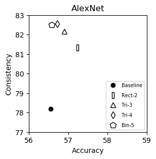
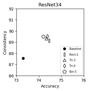
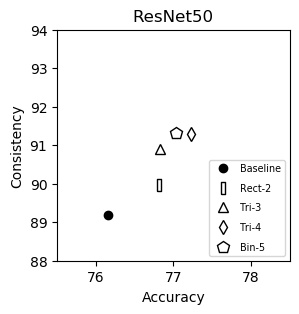
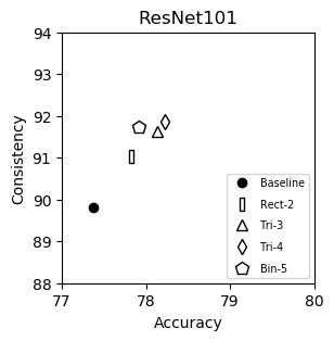
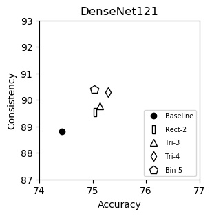
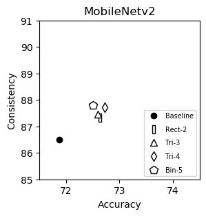
We show consistency (y-axis) vs accuracy (x-axis) for various networks. Up and to the right is good. Training and testing instructions are here.

We italicize a variant if it is not on the Pareto front -- that is, it is strictly dominated in both aspects by another variant. We bold a variant if it is on the Pareto front. We bold highest values per column.

AlexNet (plot)

	Accuracy	Consistency
Baseline	56.55	78.18
Rect-2	57.24	81.33
Tri-3	56.90	82.15
Tri-4	56.72	82.54
Bin-5	56.58	82.51

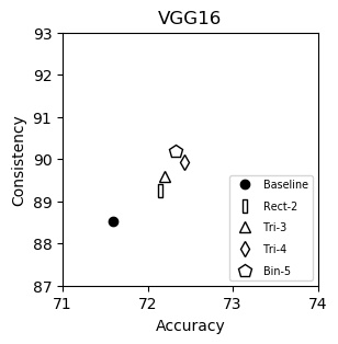
VGG16 (plot)

	Accuracy	Consistency
Baseline	71.59	88.52
Rect-2	72.15	89.24
Tri-3	72.20	89.60
Tri-4	72.43	89.92
Bin-5	72.33	90.19

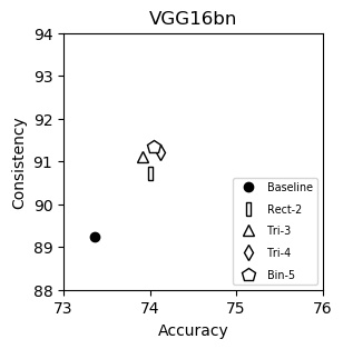
VGG16bn (plot)

	Accuracy	Consistency
Baseline	73.36	89.24
Rect-2	74.01	90.72
Tri-3	73.91	91.10
Tri-4	74.12	91.22
Bin-5	74.05	91.35

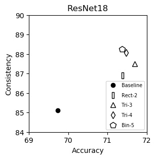
ResNet18 (plot)

	Accuracy	Consistency
Baseline	69.74	85.11
Rect-2	71.39	86.90
Tri-3	71.69	87.51
Tri-4	71.48	88.07
Bin-5	71.38	88.25

ResNet34 (plot)

	Accuracy	Consistency
Baseline	73.30	87.56
Rect-2	74.46	89.14
Tri-3	74.33	89.32
Tri-4	74.38	89.53
Bin-5	74.20	89.49

ResNet50 (plot)

	Accuracy	Consistency
Baseline	76.16	89.20
Rect-2	76.81	89.96
Tri-3	76.83	90.91
Tri-4	77.23	91.29
Bin-5	77.04	91.31

ResNet101 (plot)

	Accuracy	Consistency
Baseline	77.37	89.81
Rect-2	77.82	91.04
Tri-3	78.13	91.62
Tri-4	78.22	91.85
Bin-5	77.92	91.74

DenseNet121 (plot)

	Accuracy	Consistency
Baseline	74.43	88.81
Rect-2	75.04	89.53
Tri-3	75.14	89.78
Tri-4	75.29	90.29
Bin-5	75.03	90.39

MobileNet-v2 (plot)

	Accuracy	Consistency
Baseline	71.88	86.50
Rect-2	72.63	87.33
Tri-3	72.59	87.46
Tri-4	72.72	87.72
Bin-5	72.50	87.79

Extra Run-Time

Antialiasing requires extra computation (but no extra parameters). Below, we measure run-time (x-axis, both plots) on a forward pass of batch of 48 images of 224x224 resolution on a RTX 2080 Ti. In this case, gains in accuracy (y-axis, left) and consistency (y-axis, right) end up justifying the increased computation.

(4) Training and Evaluation

To reduce clutter, this is linked here. Help improve the results!

(A) Acknowledgments

This repository is built off the PyTorch ImageNet training and torchvision models repositories.

(B) Citation, Contact

If you find this useful for your research, please consider citing this bibtex. Please contact Richard Zhang <rizhang at adobe dot com> with any comments or feedback.