Recall that we call a tuple of puzzle pieces (P, Q) (order matters!) to be left-right adjacent if when P is placed to the left of Q, P's right edge is adjacent to Q's left edge.
We compute the left-right adjacency distance of a tuple (P,Q) as follows:
- Extract RE, the right edge of piece P (1 pixel width)
- Extract LE, the left edge of Piece Q (1 pixel width).
- Compute the difference LE-RE.
- Set the left-right adjacency distance of (P,Q) to be the euclidean norm || LE-RE||
We will use the (negative of the left-right adjacency distance ) as a score to predict the adjacency of puzzle piece tuples (P,Q)
from PIL import Image
import matplotlib.pyplot as plt
import matplotlib.ticker as plticker
import os

import pprint
import itertools
from collections import defaultdict

# generate random integer values
from random import seed
from random import randint
import numpy as np
#from pylab import array
from random import sample
import math

#pytorch modules
import torch
from torch.utils.data import Dataset, DataLoader, IterableDataset
from torchvision import transforms, utils

import sys
import Checking_adjacency_dataset as cad
%matplotlib inline
import seaborn as sns
from sklearn import metrics
Let us compute the left-right adjacency distance of puzzle piece tuples for some datapoints from our custom dataset
my_root_dir = os.getenv("MY_ROOT_DIR")
my_sq_puzzle_piece_dim = 100
my_size_of_buffer = 1000
my_model_dim = 224
my_batch_size = 20
my_adjacency_dataset = cad.AdjacencyDataset(my_root_dir, my_sq_puzzle_piece_dim,
my_size_of_buffer, my_model_dim)
my_adjacency_dataloader = DataLoader(my_adjacency_dataset, my_batch_size)Recall that a datapoint from our dataset looks like (crop(P+Q), label) where crop(P+Q) is a square piece of height = width = my_model_dim cropped from (P juxtaposed to the left of Q) containing the right edge of P and the left edge of Q in the middle
NB - We will always ensure my_model_dim is even
Since width of crop(P+Q) = my_model_dim and the labels of cols of crop(P+Q) vary from 0 to my_model_dim-1, the right edge of P is the column with label (my_model_dim//2)-1 while the left edge of Q is the column with label (my_model_dim//2)
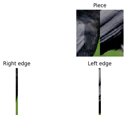
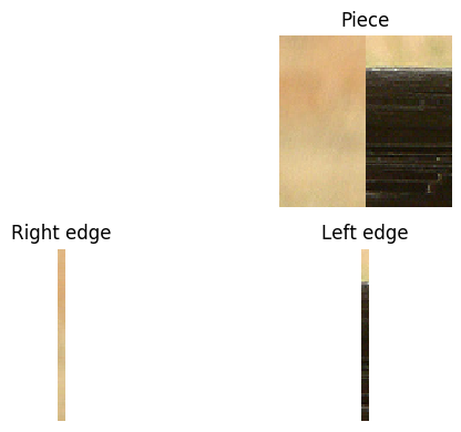
We give below a function to display edge extraction (a thickened edge is extracted for illustration. In actuality, we will extract edges of width 1 px)
def display_edge_extraction(juxtaposed_pieces_torchtensor, width):
    #batchsize x channel x height x width
    check = width % 2
    assert (check==0), "Model dim is not even"

    #Get the first piece in a batch
    piece = juxtaposed_pieces_torchtensor[0, :, :, :]

    #Extract left and right edges around middle of width 10px
    thickened_right_edge = piece[:,:,(width//2)-10:(width//2)]
    thickened_left_edge = piece[:,:,(width//2):(width//2)+10]

    #Display the extracted edges
    my_dpi = 100
    fig = plt.figure(dpi = my_dpi)

    print(f"Piece of size {piece.size()}")
    piece_image = transforms.ToPILImage()(piece)
    ax=fig.add_subplot(222)
    ax.imshow(piece_image)
    ax.title.set_text('Piece')
    plt.axis('off')

    print(f"Thickened right edge of size {thickened_right_edge.size()}")
    ax=fig.add_subplot(223)
    right_edge_image = transforms.ToPILImage()(thickened_right_edge)
    ax.imshow(right_edge_image)
    ax.title.set_text('Right edge')
    plt.axis('off')


    print(f"Thickened left edge of size {thickened_left_edge.size()}")
    ax=fig.add_subplot(224)
    left_edge_image = transforms.ToPILImage()(thickened_left_edge)
    ax.imshow(left_edge_image)
    ax.title.set_text('Left edge')
    plt.axis('off')

    fig.tight_layout()
    plt.show()
    print("*****************")
counter = 0
for juxtaposed_pieces_torchtensor, label in my_adjacency_dataloader:
    (display_edge_extraction(juxtaposed_pieces_torchtensor, my_model_dim))
    counter += 1
    if counter > 1:
        break
Piece of size torch.Size([3, 224, 224])
Thickened right edge of size torch.Size([3, 224, 10])
Thickened left edge of size torch.Size([3, 224, 10])
*****************
Piece of size torch.Size([3, 224, 224])
Thickened right edge of size torch.Size([3, 224, 10])
Thickened left edge of size torch.Size([3, 224, 10])
*****************
The following code computes the adjacency distances from a batch of cropped images (of the shape crop(P+Q))
def adjacency_dist(juxtaposed_pieces_torchtensor, width):
    #juxtaposed_pieces_torchtensor = batchsize x channel x height x width
    check = width % 2
    assert (check==0), "Model dim is not even"
    right_edges = juxtaposed_pieces_torchtensor[:, :, :, (width//2)-1]
    left_edges = juxtaposed_pieces_torchtensor[:, :, :, (width//2)]
    differences = left_edges-right_edges
    distances = torch.norm(differences, p='fro', dim=(1,2))
    return distances
no_of_batches = 0
no_of_adjacent = 0
true_labels = []
negative_distance_scores = []

for juxtaposed_pieces_torchtensor, label in my_adjacency_dataloader:
    if no_of_batches >= 500:
        break
    distances = adjacency_dist(juxtaposed_pieces_torchtensor,  my_model_dim)
    true_labels.extend(list(map(lambda x: x.item(), label)))
    negative_distance_scores.extend(list(map(lambda x: -x.item(), distances)))
    group = np.array(label)
    no_of_adjacent += np.sum(group)
    values = np.array(distances)
    p = sns.stripplot(x=group,
                      y=values,
                      jitter=0.25)
    no_of_batches += 1


total_examples = no_of_batches*my_batch_size
no_of_non_adjacent = total_examples - no_of_adjacent
print(f"Total number of examples : {total_examples}")
print(f"No of adjacent (1) labels : {no_of_adjacent}")
print(f"No of non-adjacent (0) labels : {no_of_non_adjacent}")
Total number of examples : 10000
No of adjacent (1) labels : 4580
No of non-adjacent (0) labels : 5420
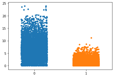
We note that for this plot the edge dimensions are 3 x 224 and each pixel entry is between 0 and 1. Thus the difference matrix (left_edge - right_edge) has dimensions 3 x 224 with entries at most 1 and at least -1. So the maximum norm of the difference is bounded above by sqrt(672) which is ~ 25.9
Eyeballing the graph, we see that adjacent tuple pieces seem to mostly have an adjacency distance of atmost 4 (ignoring outliers). However the adjaceny distance of non-adjacent tuple pieces seem to be spread out between 0 and sqrt(672) ..
In this no ML approach to checking adjacency, we would like to set a threshold distance td. We will then predict tuples with adjacency distance > td to be non-adjacent and <= td to be adjacent.
We have already computed the negative of distance scores for 5000 puzzle-piece tuples above. Recall that this data is stored in the list negative_distance_scores. For these data-points, the actual labels (adjacent(1)/non-adjacent(0)) is stored in the list true_labels
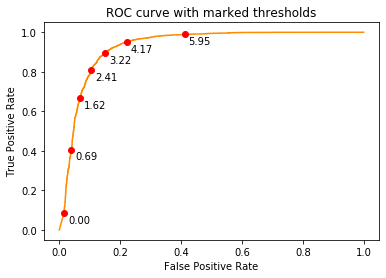
We now compute the following metrics for a range of thresholds
- False postive rate (fpr) : False positives/Total negatives
- True positive rate (tpr) or Recall: True positives/Total positives
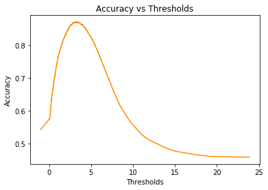
- Accuracy : True positives + True negatives/Total number of examples
- Precision : True positives/Predicted positives
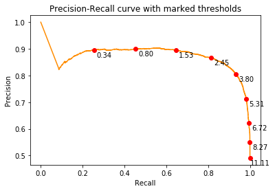
We first plot the precision-recall curve
precision, recall, prthresholds = metrics.precision_recall_curve(true_labels,negative_distance_scores, pos_label=1)
plt.figure()
plt.plot(recall,precision, color='darkorange')

for x,y,t in list(zip(recall,precision,prthresholds))[1::1000]:
    label = "{:.2f}".format(-t)
    plt.plot(x,y,"ro")
    plt.annotate(label, # this is the text
                 (x,y), # this is the point to label
                 textcoords="offset points", # how to position the text
                 xytext=(15,-10), # distance from text to points (x,y)
                 ha='center') # horizontal alignment can be left, right or center


plt.xlabel('Recall')
plt.ylabel('Precision')
plt.title('Precision-Recall curve with marked thresholds')
plt.show()
We now plot the ROC curve (fpr vs tpr)
fpr, tpr, thresholds = metrics.roc_curve(true_labels, negative_distance_scores, pos_label=1)
plt.figure()
plt.plot(fpr, tpr, color='darkorange')

for x,y,t in list(zip(fpr,tpr,thresholds))[1::300]:
    label = "{:.2f}".format(-t)
    plt.plot(x,y,"ro")
    plt.annotate(label, # this is the text
                 (x,y), # this is the point to label
                 textcoords="offset points", # how to position the text
                 xytext=(15,-10), # distance from text to points (x,y)
                 ha='center') # horizontal alignment can be left, right or center

plt.xlabel('False Positive Rate')
plt.ylabel('True Positive Rate')
plt.title('ROC curve with marked thresholds')
plt.show()
accuracy = (no_of_adjacent*tpr + (1.-fpr)*no_of_non_adjacent)/total_examplesplt.figure()
plt.plot(-1*thresholds, accuracy, color='darkorange')
plt.xlabel('Thresholds')
plt.ylabel('Accuracy')
plt.title('Accuracy vs Thresholds')
plt.show()index_of_max_accuracy = np.argmax(accuracy)threshold_for_best_accuracy = -thresholds[index_of_max_accuracy]
best_accuracy = accuracy[index_of_max_accuracy]print(f"threshold_for_best_accuracy is {threshold_for_best_accuracy}")
print(f"best_accuracy is {best_accuracy}")threshold_for_best_accuracy is 3.3036160469055176
best_accuracy is 0.8708
We set our threshold td = threshold_for_best_accuracy
Thus we predict (P,Q) to be left-right adjacent if adjacency_dist(P,Q) <= td and non-left-right-adjacent if not
negative_td= -1*threshold_for_best_accuracy
def f(score):
    if score > negative_td:
        return 1
    else:
        return 0

predicted_labels = list(map(f, negative_distance_scores))
# Confusion matrix
# The columns show the number of examples predicted for each label,
# The rows show the actual number of examples for each label.
print(metrics.confusion_matrix(true_labels, predicted_labels, labels=[1, 0]))[[4135 445]
[ 848 4572]]
# Other metrics
print(metrics.classification_report(true_labels, predicted_labels, labels=[0, 1]))
precision recall f1-score support
0 0.91 0.84 0.88 5420
1 0.83 0.90 0.86 4580
accuracy 0.87 10000
macro avg 0.87 0.87 0.87 10000
weighted avg 0.87 0.87 0.87 10000
We define our AdjacencyClassifier_NoML
class AdjacencyClassifier_NoML():
    def __init__(self,model_dim=224):
        self.model_dim=model_dim

    def negative_distance_score(self, x):
        #x dim is 3 x model_dim x mode_dim
        distances = adjacency_dist(x, self.model_dim)
        return -1*distances

    def comparison(self,d,threshold):
        ans = 1
        if d<-1*threshold:
            ans=0
        return ans

    def predictions(self,x,threshold):
        distances = self.negative_distance_score(x)
        pred = torch.tensor(list(map(lambda y: self.comparison(y,threshold),distances)))
        return pred
my_model=AdjacencyClassifier_NoML()for juxtaposed_pieces_torchtensor, label in my_adjacency_dataloader:
distances = my_model.negative_distance_score(juxtaposed_pieces_torchtensor)
print("Negative Distance scores:")
print(distances)
pred=my_model.predictions(juxtaposed_pieces_torchtensor,threshold_for_best_accuracy)
print(f"Predictions: {pred}")
print(f"Real labels : {label}")
accuracy=torch.sum(pred==label.data).item()
print(f"Accuracy : {accuracy}")
breakNegative Distance scores:
tensor([ -1.1089, -0.9075, -4.3335, -0.2143, -17.4888, -3.6755, -11.6936,
-2.4723, -0.2502, -0.9693, -3.0702, -3.0714, -2.0465, -0.7029,
-0.7742, -17.3735, -8.1539, -3.4283, -0.5818, -1.9894])
Predictions: tensor([1, 1, 0, 1, 0, 0, 0, 1, 1, 1, 1, 1, 1, 1, 1, 0, 0, 0, 1, 1])
Real labels : tensor([1, 0, 0, 1, 0, 0, 0, 0, 1, 1, 0, 0, 1, 1, 1, 0, 0, 0, 1, 0])
Accuracy : 15
