A set of python scripts to read in a electrostatic potentials and electron densities from electronic structure calculations and plot in a number of ways, including:
- Planar average
- Spherical average
- Atom centred averages
When assessing the potential utility of novel semiconducting devices (pn-juntions, heterostructures, surface terminations) through simulation, an understanding of the variation in the electrostatic potential and electron density across the system is key. However, extraction and useful presentation of this data from the raw output of the simulation (i.e. a vasp LOCPOT or CHGCAR) can prove cumbersome and often requires the use of visualisation software followed by manual data extraction. This can result in bottlenecks in high throughput screening projects, where the same data extraction procedure is repeatedly applied to large databases of candidate structures.
To address this, the Macrodensity package has been developed as a VASP, FHI-AIMS and GULP postprocessing tool. The package contains functions that enable the user to format the data from the VASP LOCPOT and CHGCAR files, the FHI-AIMS *.cube file, and GULP *.out file into physically meaningful quantities, which can then be plotted for user interpretation. So far, the code has been used to rapidly generate data for these publications: [List Publications in which Macrodensity has been used]
Matplotlib (to plot results on the fly)
ASE (for atom centred functionality)
Pandas (optional - for quicker reading speeds; requires pandas 1.2.0 or newer)
Jupyter (optional - for .ipynb notebooks in the /tutorials/)
pip install git+git://github.com/WMD-group/MacroDensity.git
- You are now ready to run the examples listed below
- If you have modified the source code, please run the unit tests with
python setup.py test.
This example is for plotting the planar average of a potential along a vector (here it is z).
The only variables which need to be set are in the first three lines. Note LOCPOT.slab file is just a regular LOCPOT grid file.
input_file = 'LOCPOT.slab'
lattice_vector = 4.75
output_file = 'planar.dat'
The variable lattice vector refers to the lattice vector of the bulk crystal structure in the direction of the plotting. It is used to get the macroscopic average, as defined in Jackson's Electrodynamics. See the heterojunction tutorial for an interactive description of this.
For the best overview of what the lattice_parameter setting should be, and how macroscopic averaging in general works, this paper from Baldereschi and the crew can't be beaten. http://iopscience.iop.org/article/10.1088/0022-3727/31/11/002/meta
The code is executed as:
python /examples/PlanarAverage.py
or alternatively, imported into another script via:
import macrodensity as md
md.plot_planar_average(lattice_vector=4.75,input_file="LOCPOT.slab",output_file="planar.dat")
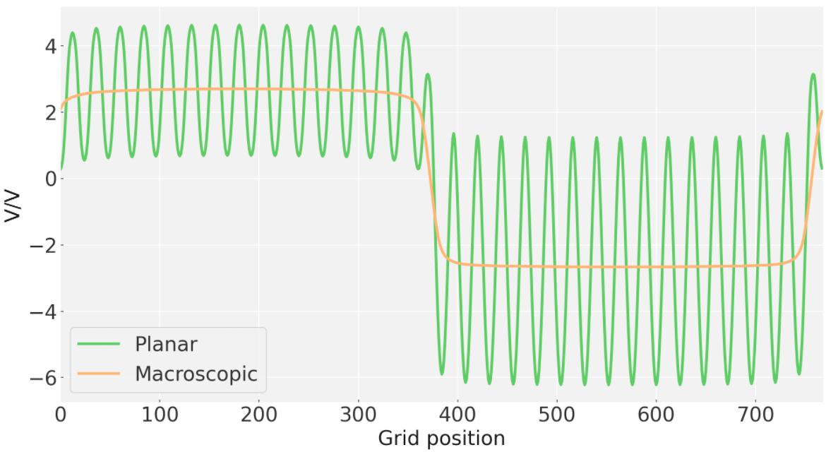
This results in a plot of the planar average and an output of the potential called planar.dat. An example of PlanarAverage.py usage is given in /tutorials/HeteroJunction/HeteroJunction.ipynb. For a ZnO/ZnS heterojunction:
The PlanarAverage.py output can be plotted as so:
Further analysis of the band offset, deformation potential and volume change is outlined in /tutorials/HeteroJunction/HeteroJunction.ipynb. For use in a slab-model style calculation for the Ionisation Potential, see /tutorials/Slab/SlabCalculation.ipynb.
This example is for plotting the average potential inside a sphere of given radius. It is the method used in our 2014 study of metal-organic frameworks in JACS.
The lines which need to be edited for this are given below. Note LOCPOT.MiL is just a regular LOCPOT file that has been renamed.
input_file = 'LOCPOT.MiL'
cube_size = [2,2,2]    # This size is in units of mesh points
## origin defines the bottom left point of the cube the "0,0,0" point in fractional coordinates
cube_origin = [0,0,0]
To run the code simply type:
python /examples/SphericalAverage.py
or alternatively, imported into another script via:
import macrodensity as md
md.spherical_average(cube_size=[2,2,2],cube_origin=[0.5,0.5,0.5],input_file='LOCPOT')
This results in an output of the average potential in the volume, and the variance of the potential:
Reading header information...
Reading 3D data using Pandas...
Average of the potential =  -8.597839951107744e-14
Potential            Variance
--------------------------------
7.145660229     2.38371017456777e-05
If the variance is too high it means that you are not sampling a plateau in the potential. Typically values below 10e-4 are acceptable, but you can also use MovingCube.py to verify this. Further examples can be found in /tutorials/Porous/Porous.ipynb
This example takes the same approach as the spherical average above, but moves the sample volume
along a defined vector. This allows you to create a 1D profile of the travelling average of the
cube. As above, all that has to be defined are the cube_size, cube_origin and input_file
parameters.
To run the code simply type:
python /examples/MovingCube.py
or alternatively, imported into another script via:
import macrodensity as md
md.moving_cube(cube=[1,1,1],vector=[1,1,1],origin=[0.17,0.17,0.17],magnitude=85,input_file='LOCPOT')
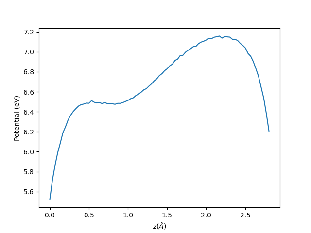
The output for a ZnS (100x100x100 FFT) unit cell is given below. The electrostatic potential at the interstices (0.5 Ang and 2.1 Ang) can be extracted using the SphericalAverage.py or bulk_interstital_alignment.
A convenience function that combines multiple instances of SphericalAverage.py, averages them and prints the Valence Band and Conduction Band positions relative ot this average. This function is based on an analysis akin to that of Frensley and Kroemer's method of band alignment. An example of its use for the ZnS (Zinc Blende) interstices is given below:
import macrodensity as md
md.bulk_interstitial_alignment(interstices=([0.5,0.5,0.5],[0.25,0.25,0.25]),outcar="OUTCAR",locpot="LOCPOT",cube_size=[2,2,2])
Data is presented in a similar format to SphericalAverage.py:
Reading header information...
Reading 3D data using Pandas...
Reading band edges from file: OUTCAR
Reading potential from file: LOCPOT
Interstital variances: [2.38371017456777e-05, 2.4181806506113166e-05]
VB_aligned      CB_aligned
--------------------------------
-4.95           -2.95
Further data gathered on Zinc Blende type structures using this function can be found here: https://aip.scitation.org/doi/10.1063/5.0044866
This example is for calculating the potential at the sites of a certain atomic nucleus, for example the O nuclei in an oxide. This on-site potential calculated this way is equivalent to a Madelung potential and can be useful for predicting electron energy levels (see http://pubs.acs.org/doi/abs/10.1021/ar400115x for details).
The input lines to edit are :
potential_file = 'LOCPOT' # The file with VASP output for potential
coordinate_file = 'POSCAR' # The coordinates file NOTE NOTE This must be in vasp 4 format
species = "O"  # The species whose on-site potential you are interested in
sample_cube = [5,5,5] # The size of the sampling cube in units of mesh points (NGX/Y/Z)
The cube parameter determines the size of the sample area, the units are mesh points, the magnitude of the mesh point is calculated by dividing the appropriate lattice vector by the number of points (NGX/Y/Z in OUTCAR).
To run the code simply type:
python /examples/OnSitePotential.py
or alternatively, imported into another script via:
import macrodensity as md
md.plot_on_site_potential(species='O',sample_cube=[5,5,5],potential_file='LOCPOT',coordinate_file='POSCAR')
The result is a histogram plot using Matplotlib. If you prefer data output simply edit the final lines of the script.
This plots the contour lines of the isosurface of an electric field in an arbitrary plane as defined in the preamble part of the file.
a_point = [0, 0, 0]
b_point = [1, 0, 1]
c_point = [0, 1, 0]

input_file = 'LOCPOT.slab'
The execution is simply:
python /examples/PlaneField.py
This creates a contour plot of the field lines.
Macrodensity also allows the facile generation of band alignment diagrams across a range of structures:
See tutorials/Plotting/Plotting.ipynb for further instructions.
Reading and manipulating electrostic potential and charge density data.
- gradient_magnitude
- vector_2_abscissa
- number_in_field
- element_vol
- one_2_2d
- macroscopic_average
- volume_average
- travelling_volume_average
- planar_average
- get_volume
- numbers_2_grid
- matrix_2_abc
- _print_boom
- read_vasp_density
- _read_partial_density
- read_vasp_parchg
- read_vasp_density_classic
- _read_vasp_density_fromlines
- density_2_grid
- density_2_grid_gulp
- read_gulp_potential
- GCD
- GCD_List
- inverse_participation_ratio
Additional tools to compliment density_tools.py
- subs_potentials
- bulk_vac
- match_resolution
- spline_generate
- matched_spline_generate
- scissors_shift
- extend_potential
- sort_potential
- diff_potentials
- translate_grid
- create_plotting_mesh
- read_cube_density
- points_2_plane
- get_third_coordinate
Convenience functions for the postprocessing and plotting of output data from density_tools.py
- bulk_interstitial_alignment
- plot_active_space
- plot_field_at_point
- plot_gulp_potential
- plot_on_site_potential
- plot_planar_average
- plot_planar_cube
- plot_plane_field
- moving_cube
- spherical_average
VASP specific tools to compliment density_tools.py
- get_band_extrema
Convenience functions for the plotting of otput data from density_tools.py
- energy_band_alignment_diagram


