A set of python scripts to read in a electrostatic potentials and electron densities from electronic structure calculations and plot in a number of ways, including:
- Planar average
- Spherical average
- Atom centred averages
When assessing the potential utility of novel semiconducting devices (pn-juntions, heterostructures, surface terminations) through simulation, an understanding of the variation in the electrostatic potential and electron density across the system is key. However, extraction and useful presentation of this data from the raw output of the simulation (i.e. a vasp LOCPOT or CHGCAR) can prove cumbersome and often requires the use of visualisation software followed by manual data extraction. This can result in bottlenecks in high throughput screening projects, where the same data extraction procedure is repeatedly applied to large databases of candidate structures.
To address this, the Macrodensity package has been developed as a VASP, FHI-AIMS and GULP postprocessing tool. The package contains functions that enable the user to format the data from the VASP LOCPOT and CHGCAR files, the FHI-AIMS *.cube file, and GULP *.out file into physically meaningful quantities, which can then be plotted for user interpretation. So far, the code has been used to rapidly generate data for these publications: 1,2
Matplotlib (to plot results on the fly)
ASE (for atom centred functionality)
Pandas (optional - for quicker reading speeds; requires pandas 1.2.0 or newer)
Jupyter (optional - for .ipynb notebooks in the tutorials)
pip install git+git://github.com/WMD-group/MacroDensity.git
- You are now ready to run the examples listed below
- If you have modified the source code, please run the unit tests with
python setup.py test.
The most widely used high level tools of macrodensity can be used as built-in convenience functions and are listed below. For finer input-control using macrodensity's lower level functions, example scripts are given in the examples folder and can be copied, modified then run via python <script.py>. Example input files can be copied from the tests folder.
Tutorials in the form of .ipynb notebooks are also given in the tutorials folder.
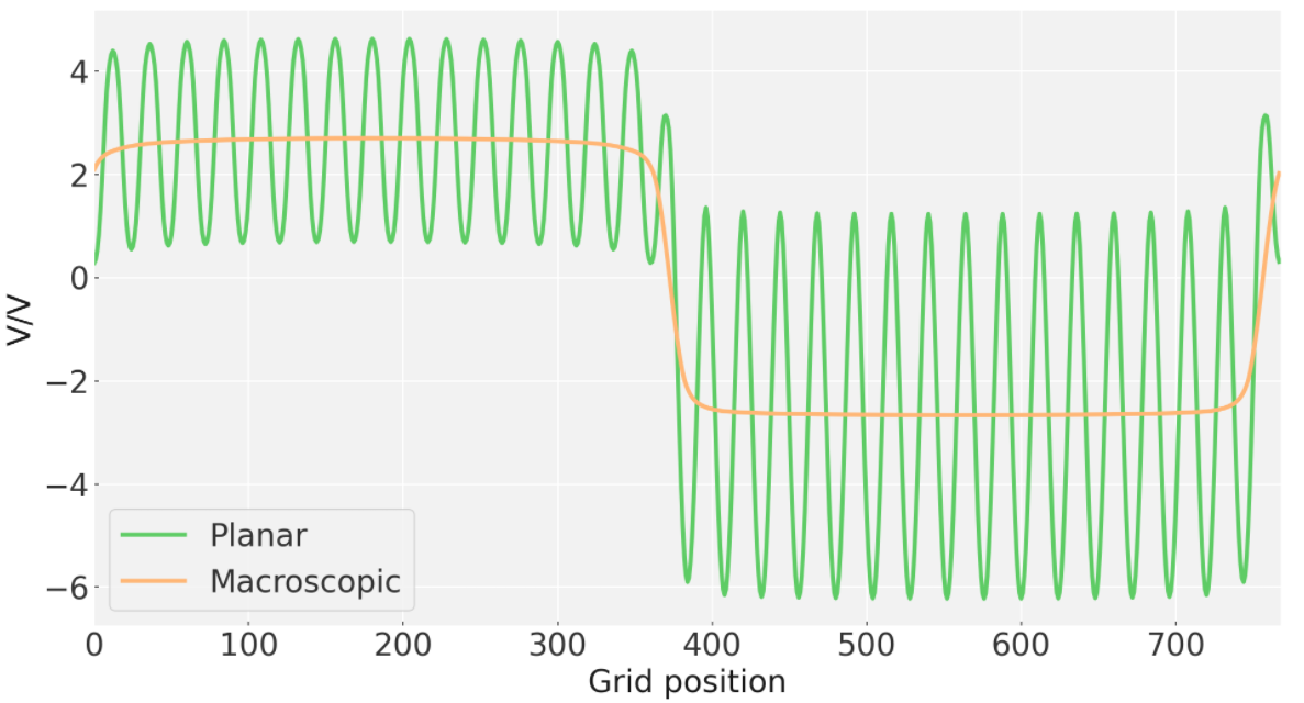
This example is for plotting the planar average and macroscopic average (as defined in Jackson's Electrodynamics) of a potential along a vector. The vector is z by default, edit examples/PlanarAverage.py to change the vector).
The function can be run via:
## Inputs:
## lattice_vector = Repeating unit over which the potential is averaged to get the macroscopic average (Angstroms)
## input_file = input filename to be read (DEFAULT = 'LOCPOT')
## output file = name of output data file (DEFAULT = 'PlanarAverage.csv')
## img_file = name of output image file (DEFAULT = 'PlanarAverage.png')

## Outputs:
## planar average and macroscopic average
## .csv data file containing: planar average and macroscopic average
## image file plotting .csv data

import macrodensity as md
md.plot_planar_average(lattice_vector=4.75, input_file='LOCPOT', output file='PlanarAverage.csv', img_file='PlanarAverage.png')
or by copying, modifying and running PlanarAverage.py separately.
For the best overview of what the lattice_vector setting should be, and how macroscopic averaging in general works, this paper from Baldereschi and the crew can't be beaten.
The output can be plotted as so:
Further analysis of the band offset, deformation potential and volume change is outlined in /tutorials/HeteroJunction/HeteroJunction.ipynb. For use in a slab-model style calculation for the Ionisation Potential, see /tutorials/Slab/SlabCalculation.ipynb.
Additionally, the planar average can be obtained and interpolated from GULP outputs:
## Inputs:
## lattice_vector = 3.0
## input_file = Name of GULP input file (DEFAULT = 'gulp.out')
## output_file = Name of output data file (DEFAULT = 'GulpPotential.csv')
## img_file = Name of output image file (DEFAULT = 'GulpPotential.png')
## new_resolution = Total number of points for the interpolated planar avarage (DEFAULT = 3000)

## Outputs:
## planar average, macroscopic average, interpolated planar average
## .csv data file containing: planar average, macroscopic average, interpolated planar average
## image file plotting .csv data

import macrodensity as md
md.plot_gulp_potential(lattice_vector=3.0, input_file='gulp.out', new_resolution = 3000)
as well as .cube files:
## Inputs:
## input_file = input filename to be read (must be in .cube format)
## lattice_vector = Repeating unit over which the potential is averaged to get the macroscopic average (Angstroms)
## output file = name of output data file (DEFAULT = 'PlanarCube.csv')
## img_file = name of output image file (DEFAULT = 'PlanarCube.png')

## Outputs:
## planar average and macroscopic average
## .csv data file containing: planar average and macroscopic average
## image file plotting .csv data

import macrodensity as md
md.plot_planar_cube(input_file='cube_file.cube', lattice_vector=4.75, output_file='PlanarCube.csv', img_file='PlanarCube.png')
See GulpPotential.py and PlanarCube.py
This example is for plotting the average potential inside a sphere of given radius. It is the method used in our 2014 study of metal-organic frameworks in JACS.
The function can be run via:
## Inputs:
## cube_size = size of the cube in units of FFT mesh points (NGX/Y/Z)
## cube_origin = real-space positioning of the bottom left point of the sampling cube (fractional coordinates of the unit cell).
## input_file = VASP LOCPOT input filename to be read (DEFAULT = 'LOCPOT')
## print_output = Print terminal output (DEFAULT = True)

## Outputs:
## cube_potential, cube_variance (Terminal)

import macrodensity as md
md.spherical_average(cube_size=[2,2,2],cube_origin=[0.5,0.5,0.5],input_file='LOCPOT')
or by copying, modifying and running SphericalAverage.py separately.
This results in an output of the average potential in the volume, and the variance of the potential:
Reading header information...
Reading 3D data using Pandas...
Average of the potential =  -8.597839951107744e-14
Potential            Variance
--------------------------------
7.145660229     2.38371017456777e-05
If the variance is too high it means that you are not sampling a plateau in the potential. Typically values below 10e-4 are acceptable, but you can also use MovingCube.py to verify this (See below). Further examples can be found in /tutorials/Porous/Porous.ipynb
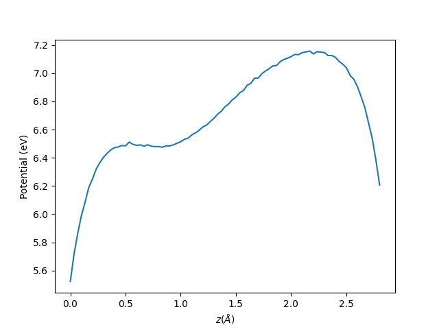
This example takes the same approach as the spherical average above, but moves the sample volume along a defined vector. This allows you to create a 1D profile of the travelling average of the cube.
The function can be run via:
## Inputs:
## cube = size of the cube in units of FFT mesh points (NGX/Y/Z)
## origin = real-space positioning of the bottom left point of the sampling cube (fractional coordinates of the unit cell).
## vector = vector across which the unit cell is traversed (hkl convention)
## magnitude = length travelled along the selected vector in units of FFT mesh points (NGX/Y/Z)
## input_file = VASP LOCPOT input filename to be read (DEFAULT = 'LOCPOT')
## output file = name of output data file (DEFAULT = 'MovingCube.csv')
## img_file = name of output image file (DEFAULT = 'MovingCube.png')

## Outputs:
## averaged electrostatic potential for the set cube size (list)
## .csv file containing the above data
## .png file presenting the above data

import macrodensity as md
md.moving_cube(cube=[1,1,1],vector=[1,1,1],origin=[0.17,0.17,0.17],magnitude=85,input_file='LOCPOT')
or by copying, modifying and running MovingCube.py separately.
The output for a ZnS (100x100x100 FFT) unit cell is given below. The electrostatic potential at the interstices (0.5 Ang and 2.1 Ang) can be extracted using SphericalAverage.py or bulk_interstital_alignment.
A convenience function that combines multiple instances of SphericalAverage.py, averages them and prints the Valence Band and Conduction Band positions relative ot this average. This function is based on an analysis akin to that of Frensley and Kroemer's method of band alignment. An example of its use for the ZnS (Zinc Blende) interstices is given below:
The function can be run via:
## Inputs:
## intersices = Positions of the pores/interstices ([[interstice1],[interstice2],...])
## outcar = VASP OUTCAR input filename (DEFAULT = OUTCAR)
## locpot = VASP LOCPOT nput filename (DEFAULT = LOCPOT)
## cube_size = a cube defined by LOCPOT FFT mesh points (DEFAULT = [2,2,2])

## Outputs:
## Aligned Valence Band, Aligned Conduction Band, Interstitial variances

import macrodensity as md
md.bulk_interstitial_alignment(interstices=([0.5,0.5,0.5],[0.25,0.25,0.25]),outcar="OUTCAR",locpot="LOCPOT",cube_size=[2,2,2])
Data is presented in a similar format to SphericalAverage.py:
Reading header information...
Reading 3D data using Pandas...
Reading band edges from file: OUTCAR
Reading potential from file: LOCPOT
Interstital variances: [2.38371017456777e-05, 2.4181806506113166e-05]
VB_aligned      CB_aligned
--------------------------------
-4.95           -2.95
Further data gathered on Zinc Blende type structures using this function can be found here
This example is for calculating the potential at the sites of a certain atomic nucleus, for example the O nuclei in an oxide. This on-site potential calculated this way is equivalent to a Madelung potential and can be useful for predicting electron energy levels (see this publication for details).
The function can be run via:
## Inputs:
## potential_file = The file with VASP output for potential (DEFAULT = 'LOCPOT')
## coordinate_file = The coordinates file (DEFAULT = 'POSCAR')
## species = The species whose on-site potential you are interested in (string)
## sample_cube = The size of the sampling cube in units of mesh points (NGX/Y/Z)
## output file = name of output data file (DEFAULT = 'OnSitePotential.csv')
## img_file = name of output image file (DEFAULT = 'OnSitePotential.png')

## Outputs:
## .png histogram output
## .csv data output

import macrodensity as md
md.plot_on_site_potential(species='O',sample_cube=[5,5,5],potential_file='LOCPOT',coordinate_file='POSCAR')
The cube parameter determines the size of the sample area, the units are mesh points, the magnitude of the mesh point is calculated by dividing the appropriate lattice vector by the number of points (NGX/Y/Z in OUTCAR).
This checks for plateaus in the electrostatic potential within a volume for a set tolerance and prints the result. cube_size defines the size of the cube in units of mesh points (NGX/Y/Z). cube_origin defines the bottom left point of the cube the "0,0,0" point in fractional coordinates.
The function can be run via:
## Inputs:
## cube_size = size of the cube in units of FFT mesh points (NGX/Y/Z)
## cube_origin = real-space positioning of the bottom left point of the sampling cube (fractional coordinates of the unit cell).
## tolerance = threshold below which the electrostatic potential is considered to be plateaued (DEFAULT = 1E-4).
## input_file = VASP LOCPOT input filename to be read (DEFAULT = 'LOCPOT')
## print_output = Print terminal output (DEFAULT = True)

## Outputs:
## Percentage of vaccum vs non-vacuum cubes

import macrodensity as md
md.plot_active_space(cube_size=[2,2,2],cube_origin=[0.5,0.5,0.5],tolerance=1E-4,input_file='LOCPOT')
Macrodensity also allows the facile generation of band alignment diagrams across a range of structures:
See tutorials/Plotting/Plotting.ipynb for further instructions.
Reading and manipulating electrostic potential and charge density data.
- gradient_magnitude
- vector_2_abscissa
- number_in_field
- element_vol
- one_2_2d
- macroscopic_average
- volume_average
- travelling_volume_average
- planar_average
- get_volume
- numbers_2_grid
- matrix_2_abc
- _print_boom
- read_vasp_density
- _read_partial_density
- read_vasp_parchg
- read_vasp_density_classic
- _read_vasp_density_fromlines
- density_2_grid
- density_2_grid_gulp
- read_gulp_potential
- GCD
- GCD_List
- inverse_participation_ratio
Additional tools to compliment density_tools.py
- subs_potentials
- bulk_vac
- match_resolution
- spline_generate
- matched_spline_generate
- scissors_shift
- extend_potential
- sort_potential
- diff_potentials
- translate_grid
- create_plotting_mesh
- read_cube_density
- points_2_plane
- get_third_coordinate
Convenience functions for the postprocessing and plotting of output data from density_tools.py
- bulk_interstitial_alignment
- plot_gulp_potential
- plot_on_site_potential
- plot_planar_average
- plot_planar_cube
- moving_cube
- spherical_average
- plot_active_space
- (under development) plot_plane_field
- (under development) plot_field_at_point
- (under development) plot_active_plane
VASP specific tools to compliment density_tools.py
- get_band_extrema
Convenience functions for the plotting of otput data from density_tools.py
- energy_band_alignment_diagram


