BBGDM is a R package for running Generalized Dissimilarity Models with Bayesian Bootstrap for parameter estimation. To install package run the following command in your R terminal
install.packages(c('devtools'))
devtools::install_github('skiptoniam/bbgdm')library(bbgdm)
library(vegan)The dune meadow vegetation data, dune, has cover class values of 30 species on 20 sites. Make the abundance data presence/absence.
data(dune)
data(dune.env)
dune_pa <- ifelse(dune>0,1,0)Now we have a species by sites matrix of vegetation data and the associated environmental data for these sites.
form <- ~1+A1
fm1 <- bbgdm(form,dune_pa, dune.env,family="binomial",link='logit',
             dism_metric="number_non_shared",spline_type = 'ispline',
nboot=100, geo=FALSE,optim.meth='nlmnib')Here we print out the basic details of the model.
print(fm1)## A Bayesian Bootstrap GDM fitted against:
## 20 sites,
## 30 species and
## 190 dissimilarities used as observations in the model.
##
## A total of 100 Bayesian Bootstraps were run.
##
## Spline base parameter estimates are:
## (Intercept) 0.6547
## x_1 0
## x_2 0.1959
## x_3 0.4745
Using the diagnostics function we can extract Random Qunatile Residuals for plotting.
resids <- diagnostics(fm1)
par(mfrow=c(2,2))
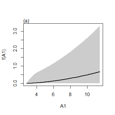
plot(resids)We can use as.response to look at the spline responses in our BBGDM. The black line represents the median fit, while the grey shaded area is the uncertainty in this fit.
response <- as.response(fm1)
par(mfrow=c(1,1))
plot(response)library(xtable)
wt <- bbgdm.wald.test(fm1)
tab <- xtable(wt)
print(tab, type = "html")| bbgdm\_W | bbgdm\_df | bbgdm\_p-value | |
|---|---|---|---|
| intercept | 11.05 | 1.00 | 0.00 |
| A1 | 1.80 | 3.00 | 0.61 |
#generate some random spatial autocorrelated data.
library(raster)
set.seed(123)
xy <- expand.grid(x=seq(145, 150, 0.1), y=seq(-40, -35, 0.1))
d <- as.matrix(dist(xy))
w <- exp(-1/nrow(xy) * d)
ww <- chol(w)
xy$z <- t(ww) %*% rnorm(nrow(xy), 0, 0.1)
xy$z <- scales::rescale(xy$z,range(dune.env$A1))
coordinates(xy) <- ~x+y
r <- rasterize(xy, raster(points2grid(xy)), 'z')
#give it the same name as variable in bbgdm model.
names(r)<- 'A1'
r2 <- raster(r)
res(r2) <- 0.05
r2 <- resample(r, r2)
#use this layer to predict turnover.
pred.dune.sim.dat <- predict(fm1,r2,uncertainty = TRUE)
## using default three cell neighbourhood to estimate dissimilarity
#plot the data and the turnover predictions, and error.
colram <- colorRampPalette(c("darkblue","yellow","red"))
colram.se <- colorRampPalette(c('antiquewhite','pink','red'))
par(mfrow=c(1,3),mar=c(3,2,2,6))
plot(r2,main='Simulated A1')
plot(pred.dune.sim.dat[[1]],col=colram(100),main='BBGDM turnover')
plot(pred.dune.sim.dat[[2]],col=colram.se(100),main='BBGDM CV of turnover')

