README.md

A ray tracer from scratch, in Haskell

This project implements a ray tracer, following the excellent book The Ray Tracer challenge, by Jamis Buck.

• Tuples, Points and Vectors
• Drawing on a canvas
• Matrices
• Matrix Transformations
• Ray-sphere intersections
• Light and Shading
• Making a scene
• Shadows
• Planes
• Patterns
• Reflection and Refraction
• Cubes
• Cylinders
• Groups
• Triangles
• Constructive Solid Geometry
• Next Steps

Tuples, Points and Vectors

Points and vectors are represented as 4-tuples of Floats, with the difference that points always end with a 1 as last coordinate, like (4, -4, 3, 1), and vectors always end with a 0.

data RTCTuple a = RTCTuple {x, y, z, w ::a} deriving (Eq, Show)

This chapter implements basic arithmetic operations on those tuples: addition, subtraction, multiplication by a scalar, approximate equality, dot product, cross product, etc...

Drawing on a canvas

Colors are introduced as (r,g,b) tuples that are Num instances, allowing some simple operations on colors:

newtype Color = Color (Float, Float, Float) deriving (Eq, Show)

instance Num Color where
    Color (r1, g1, b1) + Color (r2, g2, b2) = Color (r1 + r2, g1 + g2, b1 + b2)
    Color (r1, g1, b1) - Color (r2, g2, b2) = Color (r1 - r2, g1 - g2, b1 - b2)
    _ * _ = undefined
    abs _ = undefined
    signum _ = undefined
    fromInteger _ = undefined
    negate (Color (r, g, b)) = Color (-r, -g, -b)

From there the notion of canvas is defined as a rectangular grid of pixels:

-- Pixel matrix
type PixelMatrix = Array (Int, Int) Color

-- Canvas
newtype Canvas = Canvas PixelMatrix deriving (Show)

One can write a pixel at a given position

writePixelAt :: Canvas -> Int -> Int -> Color -> Canvas
writePixelAt (Canvas m) i j c = if (outsideCanvas i j (Canvas m)) then (Canvas m) 
    else Canvas (m // [((i,j), c)])

and also write a PPM file from a canvas, to visualize our work:

ppmFromCanvas :: Canvas -> String
ppmFromCanvas c = unlines ("P3" : [show w ++ " " ++ show h ] ++ ["255"] ++ pixelData c)
    where
        w = width c
        h = height c

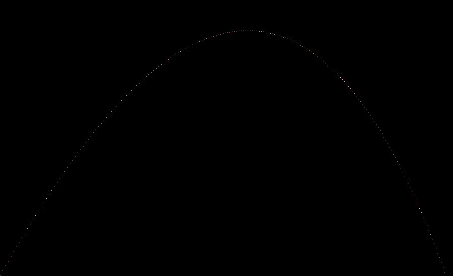
As an example, the chapter ends with the plotting of a simple parabolic trajectory:

Matrices

Matrices are introduced, with operations on them: addition, multiplication, transposition, inversion. Keeping the implementation as simple as possible I chose my matrices to be represented as arrays:

type Matrix a =  Array (Int, Int) a

Matrix transformations

In this chapter we translate, scale, rotate, shear, and chain various matrices.

Here is an example of how the rotation looks like in my implementation:

rotation_x:: Float -> Matrix Float
rotation_x r = Matrix.createMatrixFromList 4 4 [[1.0, 0.0, 0.0, 0.0::Float],
                                 [0.0, cosr, (-sinr), 0.0::Float],
                                 [0.0, sinr, cosr, 0.0::Float],
                                 [0.0, 0.0, 0.0, 1.0::Float]]
                        where cosr = cos r
                              sinr = sin r

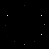
As usual, the chapter ends with a challenge: draw the 12 positions of the exact hours of a clock (using matrix rotations).

Ray-sphere intersections

Rays are created :

data Ray a = Ray {origin::RTCTuple a, direction::RTCTuple a} deriving (Eq, Show)

They can intersect spheres. First a unit sphere centered at the origin is defined. More general spheres are defined by applying transformations to that simple sphere.

data Sphere = Sphere {sphereId::Int, transform::Matrix Float, material:: Material}
  deriving (Eq,Show)

data Object = Object Sphere  deriving (Eq, Show)

sphere:: Sphere
sphere = Sphere {sphereId = 0, Sphere.transform = Matrix.identity, material = defaultMaterial}

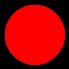
This chapter's challenge is to compute the projection of a sphere onto a wall:

Light and shading

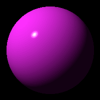
Here we implement the Phong Reflection Model and use it to render a simple sphere: