We are excited to announce PyCaret, an open source machine learning library in Python to train and deploy supervised and unsupervised machine learning models in a low-code environment. PyCaret allows you to go from preparing data to deploying models within seconds from your choice of notebook environment.
In comparison with the other open source machine learning libraries, PyCaret is an alternate low-code library that can be used to replace hundreds of lines of code with few words only. This makes experiments exponentially fast and efficient. PyCaret is essentially a Python wrapper around several machine learning libraries and frameworks such as scikit-learn, XGBoost, Microsoft LightGBM, spaCy, and many more.
PyCaret is simple and easy to use. All the operations performed in PyCaret are sequentially stored in a Pipeline that is fully orchestrated for **deployment. **Whether its imputing missing values, transforming categorical data, feature engineering or even hyperparameter tuning, PyCaret automates all of it. To learn more about PyCaret, watch this 1-minute video.
<iframe src="https://medium.com/media/a76d85d6c77246f0791956c273224c56" frameborder=0></iframe>The first stable release of PyCaret version 1.0.0 can be installed using pip. Using the command line interface or notebook environment, run the below cell of code to install PyCaret.
pip install pycaret
If you are using Azure notebooks or Google Colab, run the below cell of code to install PyCaret.
!pip install pycaret
When you install PyCaret, all dependencies are installed automatically. Click here to see the list of complete dependencies.
In this step-by-step tutorial, we will use **‘diabetes’ **dataset and the goal is to predict patient outcome (binary 1 or 0) based on several factors such as Blood Pressure, Insulin Level, Age etc. The dataset is available on PyCaret’s github repository. Easiest way to import dataset directly from repository is by using **get_data **function from pycaret.datasets modules.
from **pycaret.datasets** import **get_data**
diabetes = **get_data**('diabetes')
💡 PyCaret can work directly with pandas dataframe.
The first step of any machine learning experiment in PyCaret is setting up the environment by importing the required module and initializing setup( ). The module used in this example is **pycaret.classification.**
Once the module is imported, **setup() **is initialized by defining the dataframe (‘diabetes’) and the target variable (‘Class variable’).
from **pycaret.classification** import ***
**exp1 = **setup**(diabetes, target = 'Class variable')
All the preprocessing steps are applied within **setup(). **With over 20 features to prepare data for machine learning, PyCaret creates a transformation pipeline based on the parameters defined in *setup *function. It automatically orchestrates all dependencies in a **pipeline **so that you don’t have to manually manage the sequential execution of transformations on test or unseen dataset. PyCaret’s pipeline can easily be transferred across environments to run at scale or be deployed in production with ease. Below are preprocessing features available in PyCaret as of its first release.
💡 Data Preprocessing steps that are compulsory for machine learning such as missing values imputation, categorical variable encoding, label encoding (converting yes or no into 1 or 0), and train-test-split are automatically performed when setup() is initialized. Click here to learn more about PyCaret’s preprocessing abilities.
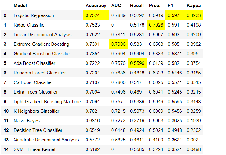
This is the first step recommended in supervised machine learning experiments (classification or regression). This function trains all the models in the model library and compares the common evaluation metrics using k-fold cross validation (by default 10 folds). The evaluation metrics used are:
-
**For Classification: **Accuracy, AUC, Recall, Precision, F1, Kappa
-
**For Regression: **MAE, MSE, RMSE, R2, RMSLE, MAPE
compare_models()
💡 Metrics are evaluated using 10-fold cross validation by default. It can be changed by changing the value of ***fold ***parameter.
💡 Table is sorted by ‘Accuracy’ (Highest to Lowest) value by default. It can be changed by changing the value of ***sort ***parameter.
Creating a model in any module of PyCaret is as simple as writing *create_model. ***It takes only one parameter i.e. the model name passed as string input. This function returns a table with k-fold cross validated scores and a trained model object.
adaboost = **create_model**('ada')
Variable ‘adaboost’ stores a trained model object returned by create_model function is a scikit-learn estimator. Original attributes of a trained object can be accessed by using *period ( . ) *after variable. See example below.
💡 PyCaret has over 60 open source ready-to-use algorithms. Click here to see a complete list of estimators / models available in PyCaret.
The **tune_model function is used for automatically tuning hyperparameters of a machine learning model. **PyCaret uses random grid search over a predefined search space. This function returns a table with k-fold cross validated scores and a trained model object.
tuned_adaboost = tune_model('ada')
💡 The **tune_model **function in unsupervised modules such as pycaret.nlp, pycaret.clustering and pycaret.anomaly can be used in conjunction with supervised modules. For example, PyCaret’s NLP module can be used to tune number of topics parameter by evaluating an objective / cost function from a supervised ML model such as ‘Accuracy’ or ‘R2’.
The **ensemble_model function is used for ensembling trained models. **It takes only one parameter i.e. a trained model object. This functions returns a table with k-fold cross validated scores and a trained model object.
# creating a decision tree model
dt = **create_model**('dt')

# ensembling a trained dt model
dt_bagged = **ensemble_model**(dt)
💡 ‘Bagging’ method is used for ensembling by default which can be changed to ‘Boosting’ by using the method parameter within the ensemble_model function.
💡 PyCaret also provide blend_models and stack_models functionality to ensemble multiple trained models.
Performance evaluation and diagnostics of a trained machine learning model can be done using the **plot_model **function. It takes a trained model object and the type of plot as a string input within the plot_model function.
# create a model
adaboost = **create_model**('ada')

# AUC plot
**plot_model**(adaboost, plot = 'auc')

# Decision Boundary
**plot_model**(adaboost, plot = 'boundary')

# Precision Recall Curve
**plot_model**(adaboost, plot = 'pr')

# Validation Curve
**plot_model**(adaboost, plot = 'vc')
Click here to learn more about different visualization in PyCaret.
Alternatively, you can use **evaluate_model **function to see plots *via *user interface within notebook.
**evaluate_model**(adaboost)
💡 plot_model function in **pycaret.nlp **module can be used to visualize text corpus and semantic topic models. Click here to learn more about it.
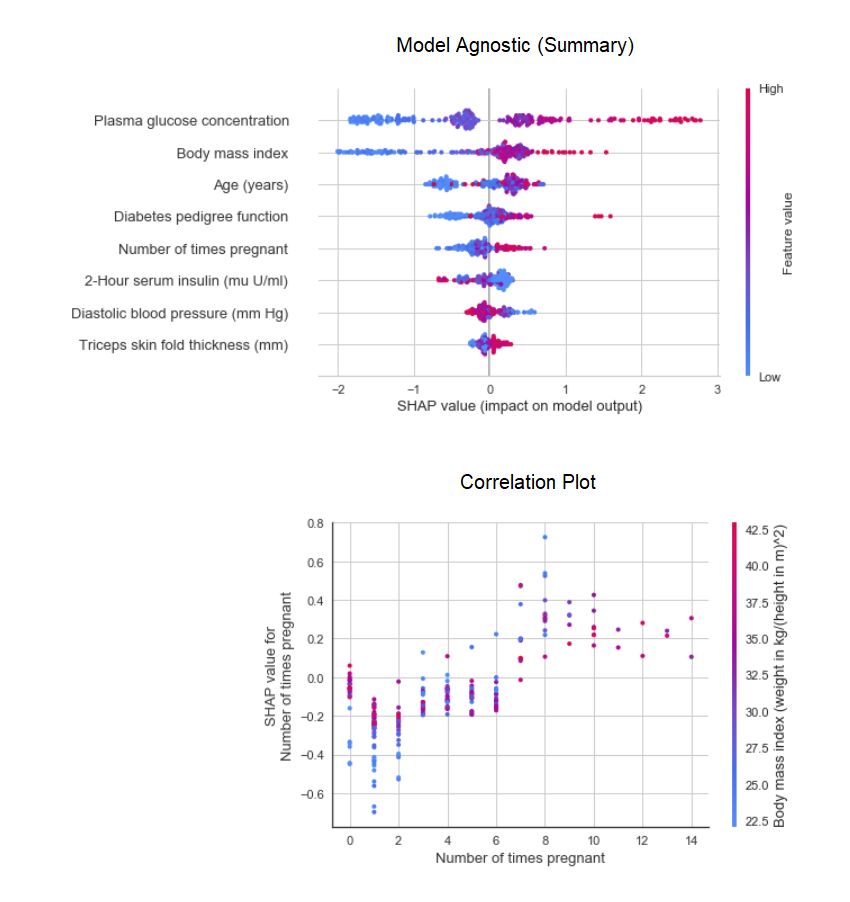
When the relationship in data is non-linear which is often the case in real life we invariably see tree-based models doing much better than simple gaussian models. However, this comes at the cost of losing interpretability as tree-based models do not provide simple coefficients like linear models. PyCaret implements SHAP (SHapley Additive exPlanations using **interpret_model **function.
# create a model
xgboost = **create_model**('xgboost')

# summary plot
**interpret_model**(xgboost)

# correlation plot
**interpret_model**(xgboost, plot = 'correlation')
Interpretation of a particular datapoint (also known as reason argument) in the test dataset can be evaluated using ‘reason’ plot. In the below example we are checking the first instance in our test dataset.
**interpret_model**(xgboost, plot = 'reason', observation = 0)
So far the results we have seen are based on k-fold cross validation on training dataset only (70% by default). In order to see the predictions and performance of the model on the test / hold-out dataset, the predict_model function is used.
# create a model
rf = **create_model**('rf')

# predict test / hold-out dataset
rf_holdout_pred **= predict_model**(rf)
**predict_model **function is also used to predict unseen dataset. For now, we will use the same dataset we have used for training as a *proxy *for new unseen dataset. In practice, **predict_model **function would be used iteratively, every time with a new unseen dataset.
predictions = **predict_model**(rf, data = diabetes)
💡 predict_model function can also predict a sequential chain of models which are created using stack_models and create_stacknet function.
💡 predict_model function can also predict directly from the model hosted on AWS S3 using deploy_model function.
One way to utilize the trained models to generate predictions on an unseen dataset is by using the predict_model function in the same notebooks / IDE in which model was trained. However, making the prediction on an unseen dataset is an iterative process; depending on the use-case, the frequency of making predictions could be from real time predictions to batch predictions. PyCaret’s deploy_model function allows deploying the entire pipeline including trained model on cloud from notebook environment.
**deploy_model**(model = rf, model_name = 'rf_aws', platform = 'aws',
             authentication =  {'bucket'  : 'pycaret-test'})
Once training is completed the entire pipeline containing all preprocessing transformations and trained model object can be saved as a binary pickle file.
# creating model
adaboost = **create_model**('ada')

# saving model**
save_model**(adaboost, model_name = 'ada_for_deployment')
You can also save the entire experiment consisting of all intermediary outputs as one binary file.
**save_experiment**(experiment_name = 'my_first_experiment')
💡 You can load saved model and saved experiment using **load_model **and **load_experiment **function available in all modules of PyCaret.
In the next tutorial, we will show how to consume a trained machine learning model in Power BI to generate batch predictions in a real production environment.
Please also see our beginner level notebooks for these modules:
Regression Clustering Anomaly Detection Natural Language Processing Association Rule Mining
We are actively working on improving PyCaret. Our future development pipeline includes a new **Time Series Forecasting **module, Integration with **TensorFlow **and major improvements on scalability of PyCaret. If you would like to share your feedback and help us improve further, you may fill this form on website or leave a comment on our GitHub or LinkedIn page.
As of the first release 1.0.0, PyCaret has the following modules available for use. Click on the links below to see the documentation and working examples.
Classification Regression Clustering Anomaly Detection Natural Language Processing Association Rule Mining
User Guide / Documentation Github Repository Install PyCaret Notebook Tutorials Contribute in PyCaret
Give us ⭐️ on our github repo if you like PyCaret.
To hear more about PyCaret follow us on LinkedIn and Youtube.


