Deep learning Dynamic MRI Reconstruction

ShanghaiTech BME1312 24 spring project1

If you think the project is inspirational or interesting, please give it a star.

Quick Start

1. Download the dataset You can download the dataset from here

2. Install necessary packages

• torch
• tensorboard
• numpy
• torchvision
• matplotlib

3. Train and test

    To run the code, you should enter the following sentences in the terminal:

python train.py output_folder
#output folder is a parameter you can randomly choose

    After running the above code, you can get undersampling, full sampling, and reconstruction images separately in different folders and a file called output.txt in which the values of loss, PSNR, and SSIM are.

    Besides, you can change the parameter value setting in train.py. Below are our default settings:

train(in_channels=20,
      out_channels=20,
      init_features=64,
      num_epochs=400,
      weight_decay=1e-4,
      batch_size=10,
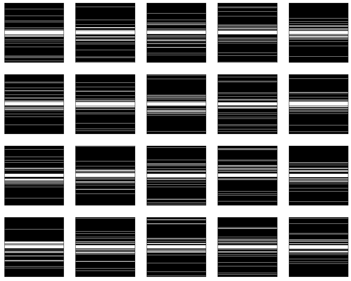
      initial_lr=1e-4)

Main idea

1. Accelerated Cine Imaging with Aliasing

The undersampling mask is generated separately for each dynamic frame. We can run the the following code to get the 20 frames dynamic image mask.

from CS_mask import cartesian_mask
mask = cartesian_mask(shape=(1, 20, 192, 192), acc=6, sample_n=10, centred=True)
imsshow(mask[0, :, :, :], num_col=5, cmap='gray')

The output is in Graph 1.1. We can clearly see that the undersampling mask for dynamic frames differs.

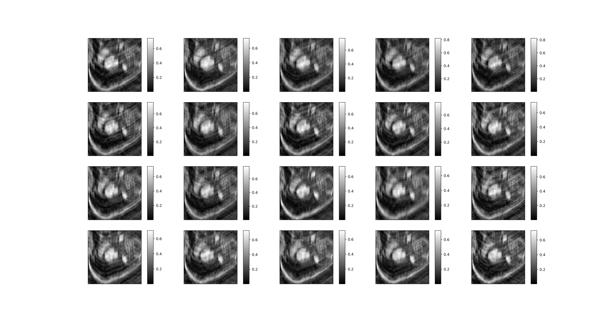
Then, we can obtain the aliased images as a result of undersampling with the generated patterns, according to the formula: $b=F^{-1}UFm$, where $m$ is the fully sampled image, $U$ is the corresponding undersampling pattern, $F$ is the Fourier transform and $b$ is the aliased image.

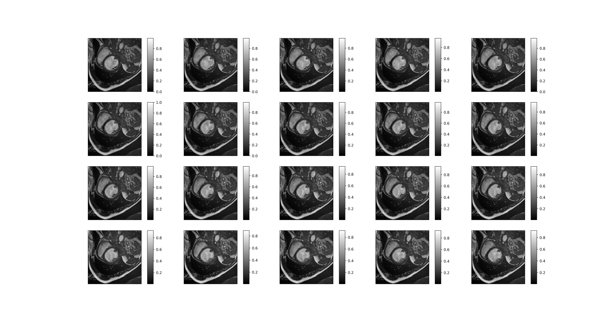
The aliased images(Graph 1.2) and fully sampled images (Graph 1.3) are as follows.

Graph 1.1 undersampling mask for different dynamic frames
Graph 1.2 Aliased images
Graph 1.3 fully sampled image

2. Basic Network

Our dataset cine. npz is a fully sampled cardiac cine MR image with the size of [nsamples, nt, nx, ny]

• nsamples = 200 is the total number of data samples
• nt is the number of dynamic frames
• nx, ny indicate the size of each 2D dynamic image, respectively.

CS_mask.py: generates 2D variable-density undersampling masks for a dynamic sequence.

train.py: training and testing the network.

We split the cine dataset into training, validation, and testing with a ratio of 4:1:2, which is 114, 29, and 57 separately. The code is as follows.

train_size = 114
val_size = 29
test_size = 57
train_set, val_set, test_set = torch.utils.data.random_split(dataset, [train_size, val_size, test_size])
    dataloader_train = DataLoader(train_set, batch_size=batch_size, shuffle=True)
    dataloader_val = DataLoader(val_set, batch_size=batch_size, shuffle=True)
    dataloader_test =  DataLoader(test_set, batch_size=batch_size, shuffle=True)

To explore the temporal correlation, we choose to stack the dynamic images along the channel dimension so that the input dimension is 20, which is the frames of the dynamic image. By the way, we have tried 3D CNN. But it's so memory-consuming that we finally give up this idea.

However, Stacking also brings some problems. The image is pseudo-complex, which means each frame has two dimensions. Thus, it's strange to stack them directly to utilize temporal correlation. After several trials, we find processing the real part and the Imaginary part works best.

We choose U-Net as the backbone and the model is as follows:

Noticed that the two U-Net don't share parameters because it will decrease the performance of the model. The reason for that may be the Peculiarities of data.

However, we find that the performance of our model is not good enough. Also, the training loss and eval loss are very close, which shows that our model may be more complex to improve the performance. Instead of only increasing the parameters of U-Net, we add another ResNet network after getting the Ouptut of U-Net. The final model is as follows:

The best performance of our model is as follows:

Loss	Avg PSNR	Std PSNR	Avg SSIM	Std SSIM
0.00166	28.214	2.057	0.815	0.035

A good reconstructed dynamic image is as follows:

Before reconstruction
After reconstruction

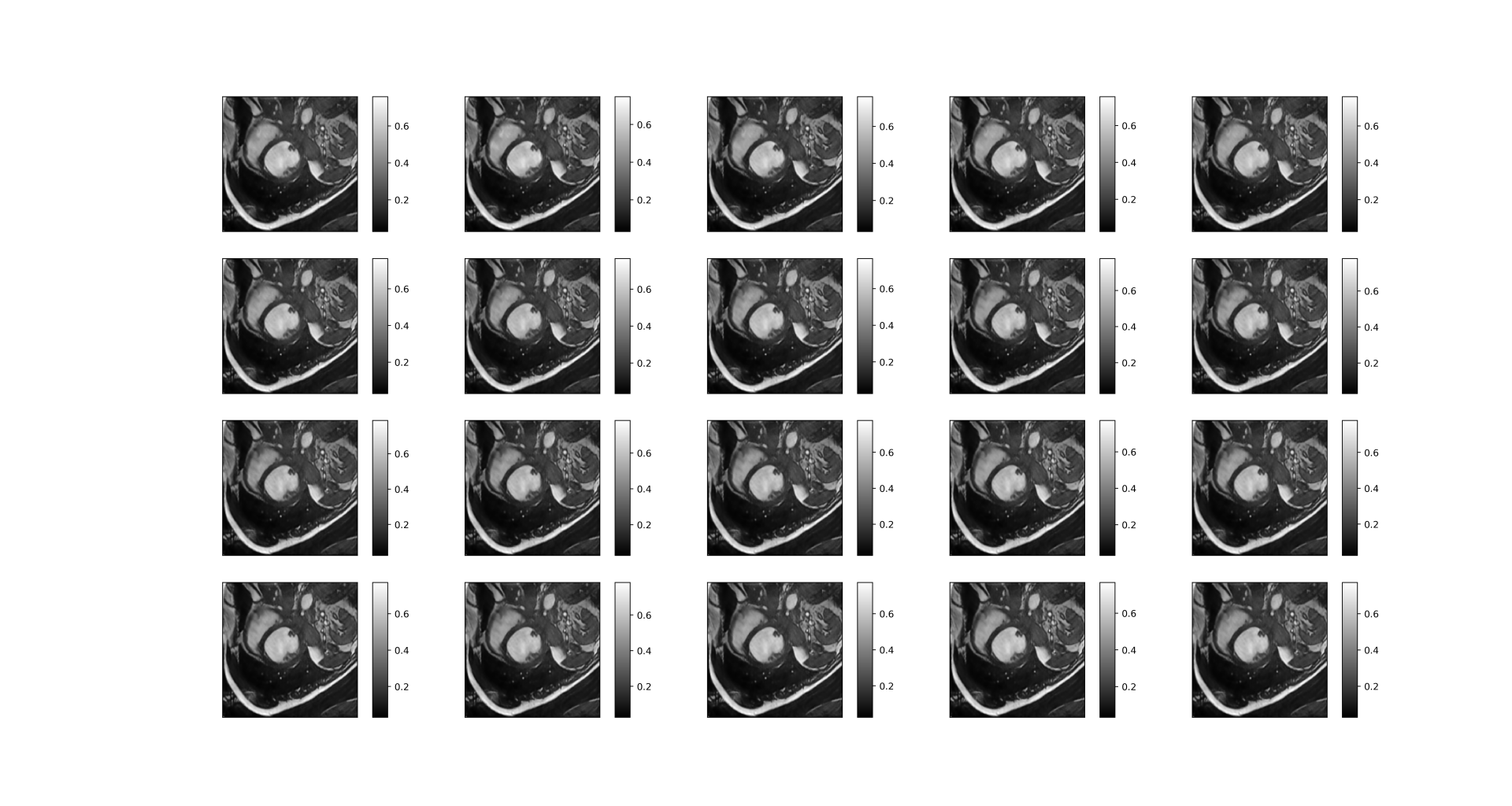We can see that the reconstructed image is very clear with many details, though the upper right corner of the picture is slightly blurry.

3. Optimization Techniques

Dropout is a widely used regularization technique in neural networks to prevent overfitting. Adding dropout will improve the network's generalization ability, making it perform better on unseen data. We also tried to add dropout to our model. However, it doesn't work well. It ruined the performance of our model. We guess it‘s because the images in the dataset have a similar distribution. Thus, a model without strong regularization can also work well and dropout even disturbs the training process which makes the network hard to train.

At the same time, we tried data augmentation. However, it doesn't work well, too. The code is as follows:

def apply_transforms(x):
    batch_size, num_samples, channels, height, width = x.size()
    x_flat = x.view(-1, channels, height, width)
    transformed_samples = []
    for sample in x_flat:
        sample_pil = transforms.ToPILImage()(sample)
        sample_transformed = transforms.Compose([
            transforms.Grayscale(num_output_channels=1),
            transforms.RandomHorizontalFlip(p=0.5),
            transforms.ColorJitter(brightness=0.2, contrast=0.2, saturation=0.2, hue=0.1),
            transforms.RandomApply([transforms.GaussianBlur(kernel_size=5, sigma=(0.1, 2.0))], p=0.5),
            transforms.RandomAffine(degrees=10, translate=(0.1, 0.1), scale=(0.9, 1.1), shear=5),
            transforms.ToTensor()
        ])(sample_pil)
        transformed_samples.append(sample_transformed)
    transformed_x = torch.stack(transformed_samples).view(batch_size, num_samples, channels, height, width)
    return transformed_x

We tried single and many combinations of these transformations but there is not even one transformation that finally improves the performance of our model. We suspect that the dataset is small and such transformations make the model harder to capture the features of images, which decreases the performance.

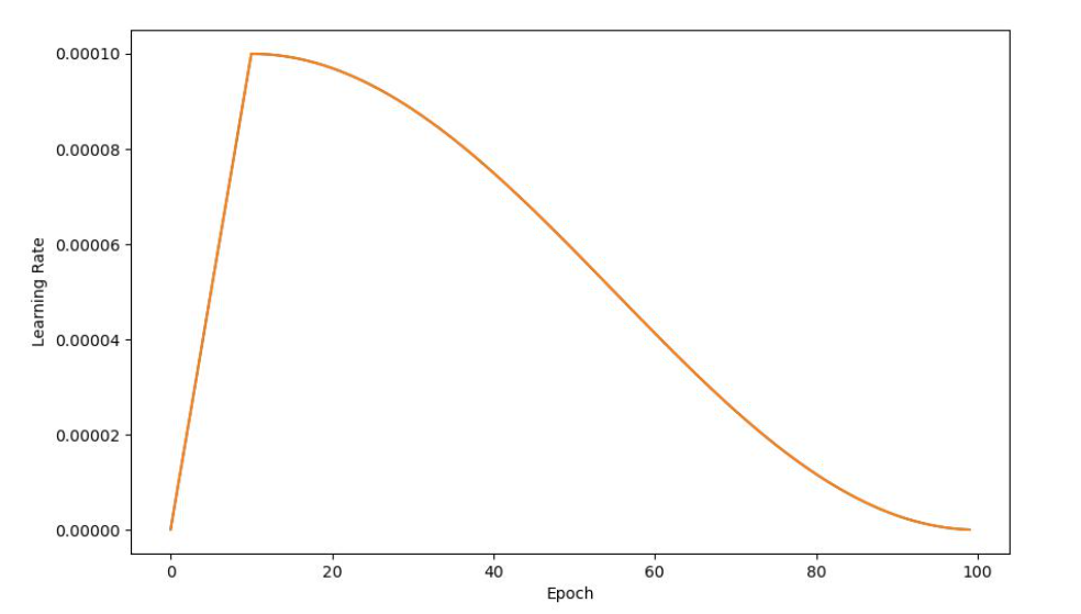
Later, we tried a dynamic learning rate. We Let the model warm up in the first 10 epochs and then Cosine Anneal. The graph of the learning rate is as follows:

Learning rate is a hyperparameter that determines the size of the steps taken during the optimization process of training a neural network. Dynamic learning rates make the learning process more stable and Ultimately converge to a very low loss. If we use a constant learning rate, In the later stages of learning, the loss curve may oscillate and be difficult to converge.

We also introduce Batch normalization to our model. It improves the training speed, stability, and performance. Because removing Batch normalization makes our model very hard to train, we consider Batch normalization as a default setting in the following experiment. It means that the model without optimization also contains Batch normalization. The experiments are as follows:

	Loss	PSNR	SSIM
Without optimization	0.00226	26.921	0.770
With weight decay	0.00205	27.399	0.774
With dropout	0.00239	26.426	0.739
With dynamic learning rate	0.00198	27.493	0.780

These experiments investigate the inflation of a single technique. It shows that both weight decay and dynamic learning rate help to improve the performance of the model, while only dropout decreases the performance.