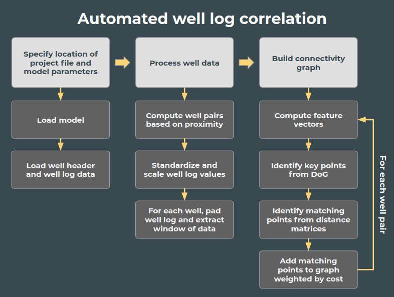
This repository contains a preliminary (and admittely incomplete) set of scripts that can be used to correlate two or more well logs automatically without any user input.
Well log correlation is the process of identifying equivalent geological units / features between two or more well logs. This is commonly done by identifying corresponding patterns between well logs from different wells and assigning them to a particular marker. This process allows us to develop an understanding of the subsurface geology and answer a variety of different questions.
Correlating well logs is a time consuming, tedious task. Depending on the number of wells, number of formations that are being interpreted, quality of the data, and the complexity of the geology this process can take days to months to complete. Additionally, this process is susceptible to bias as we each bring our own individual background and experiences, as well as prone to error as there is ambiguity in the well logs and general complexity of correlation.
The process captured in this repository leverages a variety of different capabilities from the computer vision and image processing community. Essentially, the approach outlined here is a 1D adaptation of panoramic stiching using feature vectors generated from a 1D Convolutional Autoencoder. The basic idea being to identify a series of matching points between a pair of well logs from locally minimal values in a cost matrix that was generated from two sets of feature vectors.
Ultimately we want to train a model that can learn higher dimensional representations of well log expressions that we can use to assess similarities between well logs. In order to achieve this a very simple 1D Convolutional Autoencorder was put together using PyTorch. This model contains a 5 layer enconding method consiting of 1D convolutional layers that are combined with ReLu activation and Max Pooling functions, as well as a 5 layer decoding method consisting of 1D transpose convolutional layers that are combined with ReLu activation functions. There is definitely room to improve on the architecture of this model.
Aggregate as many well logs of the same type as possible and put them in the same directory. The createTrainingData.py script accepts a series of command line arguements that will process the well log data and for each well take a series of windowed extractions and save them to disk as a 2D array. Explaination of the arguements can be found in the script. An example would be:
python createTrainingData.py --data-name autoWell --data-dir /path/to/LAS/files --output-dir /path/to/save/to --log-name GR
Training the model is fairly simple and consistent with how most CNN's are trained. The trainModel.py script accepts a series of command line arguements that will being the training process. Explaination of the arguements can be found in the script. An example would be:
python trainModel.py --model-name myNewModel --data-dir /path/to/trainingData --output-dir /location/to/save/model
Note: The model doesn't always initialize well. If the loss remains fairly consistent after a few epochs, kill the script and run again
Note: Currently the script is hard coded in terms of optimizer, learning rate, and criterion
Here is an example of the prediction on a windowedd extraction from the test data set along with the loss curves after nearly 250 epochs.

In order to correlate well logs using these scripts you will need to create a project file. This file is a HDF5 data store that contains the well header and all of the well logs as Pandas DataFrames.
Creating the project is a bit clunky, but using the createAutoWellProject.py script along with the appropriate command line arguements you should be able to successfully construct a project. In the header file you will need to have at least 3 columns, 1) UWI / API, 2) X coorinate, and 3) Y coordinate. In the terminal you will need to specify the column name that corresponds to the appropriate value so the script will use the right columns. Additionally, the LAS files must be named the same value as can be found in the UWI column of the header to match the well log data to the appropriate coordinate. Explaination of the arguements can be found in the script. An example would be:
python createAutoWellProject.py --proj-name autoWell --proj-dir /path/to/project/location --header-dir /path/to/headerFile --las-dir /las/directory --uwi-col APINo --x-col Longitude --y-col Latitude
The correlation process is an adaptation of panormic stiching for 1D well logs. The scripts provided here are somewhat incomplete. Please see the end of the README file for additional work.
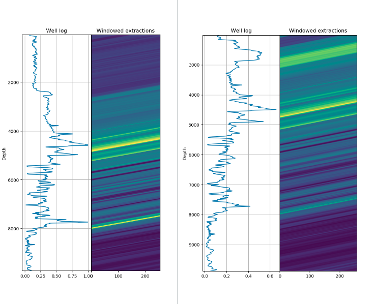
The first two steps are relatively straight forward. We first need to load the data and process the well logs to be usable by our 1D Convolutional Autoenconder. Additionally, we identify well pairs based on spatial proximity to each other.
An example of what the windowed well log data looks like:
To automatically correlate our well logs we iterate over all of the pairs of wells and process the pairs individually.
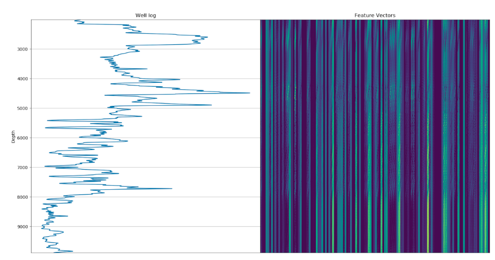
First, we compute the feature vectors by passing the well log values through encoding portion of our autoencoder:
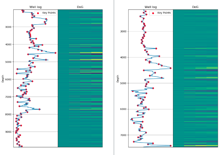
Second, we compute the Difference of Gaussians and identify key points for each well log:
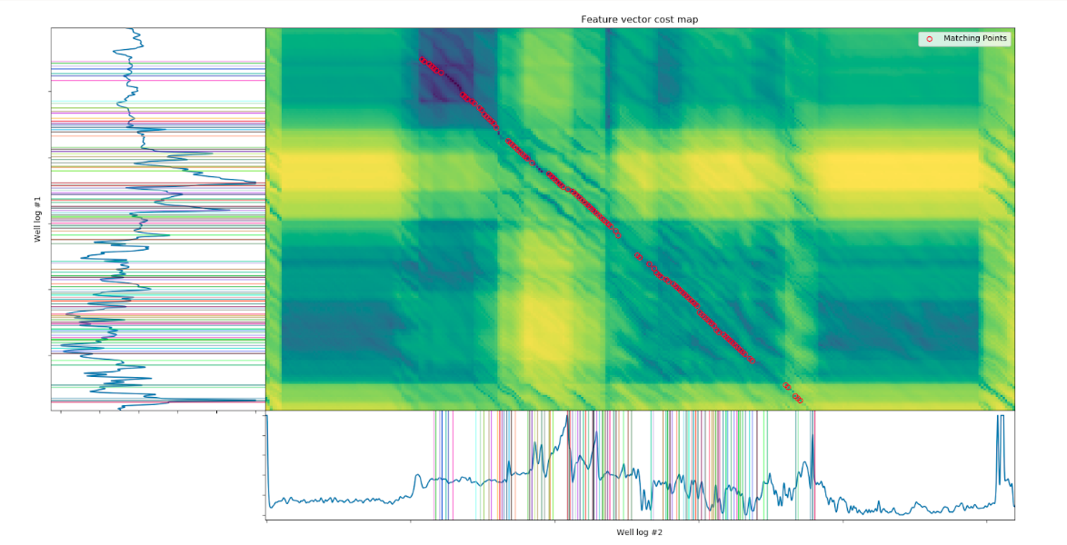
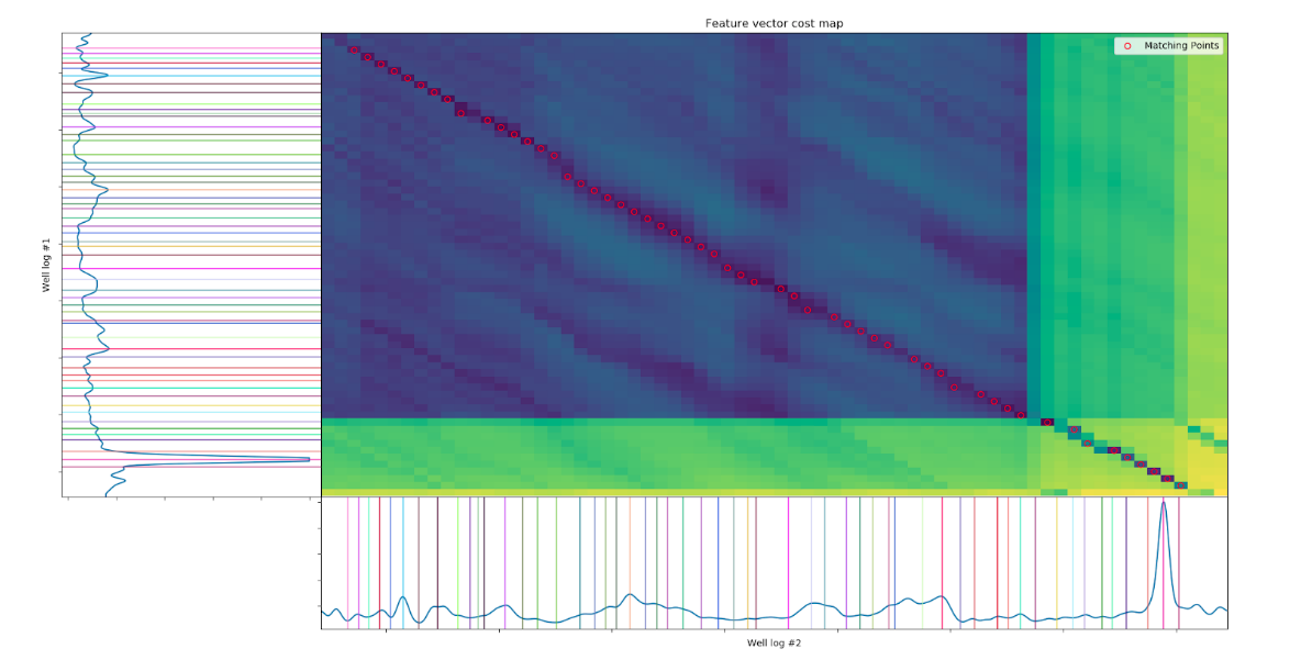
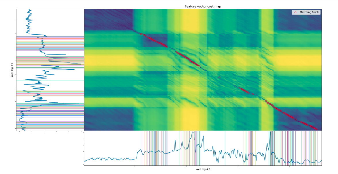
Third, we compute a cost and a lag (depth) distance matrix using the feature vectors and depths at the location of the key points identified in the previous step. The cost matrix is then analyzed for local minima in both the I and J directions to find matching points which represent the indices of correlations between well logs
Example of cost map and matching points:
Each of the matching points is added to a NetworkX graph as an edge. The purpose of generating this graph is to enable automated picking of individual markers or for generating a global interpretation across all wells and depths. The results here are limited, but could be extended to encompass the global solution.


