水文气象中推荐使用Mann-Kendall趋势检验
这是一种非参数统计检验方法,在中心趋势不稳定时,关注数据的秩。
该方法不需要不需要满足正态分布的假设,因而具有普适性。
根据自己需要(图像、并行计算、线趋势图等等)分享python\matlab\R的方法
代码如下:
# -*- coding: utf-8 -*-

from __future__ import division
import numpy as np
import pandas as pd
from scipy import stats
from scipy.stats import norm

def mk_test(x, alpha=0.05):
    """
    This function is derived from code originally posted by Sat Kumar Tomer
    ([email protected])
    See also: http://vsp.pnnl.gov/help/Vsample/Design_Trend_Mann_Kendall.htm
    The purpose of the Mann-Kendall (MK) test (Mann 1945, Kendall 1975, Gilbert
    1987) is to statistically assess if there is a monotonic upward or downward
    trend of the variable of interest over time. A monotonic upward (downward)
    trend means that the variable consistently increases (decreases) through
    time, but the trend may or may not be linear. The MK test can be used in
    place of a parametric linear regression analysis, which can be used to test
    if the slope of the estimated linear regression line is different from
    zero. The regression analysis requires that the residuals from the fitted
    regression line be normally distributed; an assumption not required by the
    MK test, that is, the MK test is a non-parametric (distribution-free) test.
    Hirsch, Slack and Smith (1982, page 107) indicate that the MK test is best
    viewed as an exploratory analysis and is most appropriately used to
    identify stations where changes are significant or of large magnitude and
    to quantify these findings.
    Input:
        x:   a vector of data
        alpha: significance level (0.05 default)
    Output:
        trend: tells the trend (increasing, decreasing or no trend)
        h: True (if trend is present) or False (if trend is absence)
        p: p value of the significance test
        z: normalized test statistics
    Examples
    --------
      >>> x = np.random.rand(100)
      >>> trend,h,p,z = mk_test(x,0.05)
    """
    n = len(x)
    # calculate S
    s = 0
    for k in range(n - 1):
        for j in range(k + 1, n):
            s += np.sign(x[j] - x[k])

    # calculate the unique data
    unique_x, tp = np.unique(x, return_counts=True)
    g = len(unique_x)

    # calculate the var(s)
    if n == g:  # there is no tie
        var_s = (n * (n - 1) * (2 * n + 5)) / 18
    else:  # there are some ties in data
        var_s = (n * (n - 1) * (2 * n + 5) - np.sum(tp * (tp - 1) * (2 * tp + 5))) / 18

    if s > 0:
        z = (s - 1) / np.sqrt(var_s)
    elif s < 0:
        z = (s + 1) / np.sqrt(var_s)
    else:  # s == 0:
        z = 0

    # calculate the p_value
    p = 2 * (1 - norm.cdf(abs(z)))  # two tail test
    h = abs(z) > norm.ppf(1 - alpha / 2)

    if (z < 0) and h:
        trend = 'decreasing'
    elif (z > 0) and h:
        trend = 'increasing'
    else:
        trend = 'no trend'

    return trend, h, p, z


df = pd.read_csv('../GitHub/statistic/Mann-Kendall/data.csv')
trend1, h1, p1, z1 = mk_test(df['data'])
上述代码太麻烦了,推荐使用pymannkendall包,只需要两行:
import pymannkendall as mk
result = mk.original_test(df['data'], alpha=0.05)
result
结果如图:

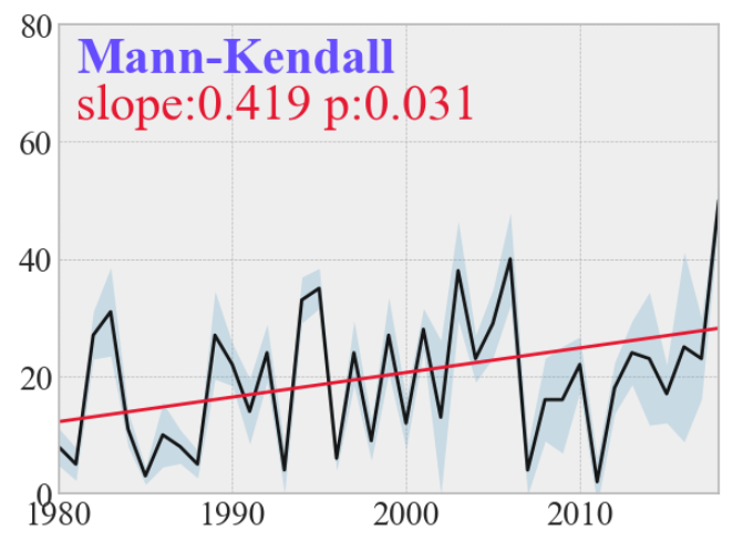
根据结果绘图(还是上述数据):
import matplotlib.pyplot as plt
import cmaps
import seaborn as sns
palette = cmaps.Cat12_r
plt.style.use('bmh')
plt.figure(figsize=(7, 5))
plt.plot(df['x'], df['data'], marker='', color='black', linewidth=2, alpha=0.9)
a = result[7]; b = result[8]; p = result[2]
y1 = a * (df['x'].values - 1979) + b
plt.plot(df['x'], y1, lw=2, color=palette(0))
plt.fill_between(df['x'], df['data'] - df['std'], df['data'] + df['std'], alpha=.2, linewidth=0)
plt.tick_params(labelsize=20)
sns.set_theme(font='Times New Roman')
plt.text(1981, 80*9/10, 'Mann-Kendall', fontweight='heavy', color=palette(2), fontsize=30)
plt.text(1981, 80*8/10, 'slope:'+str(a)[0:5]+' p:'+str(p)[0:5], color=palette(0), fontsize=30)
plt.xlim(1980, 2018)
plt.ylim(0, 80)
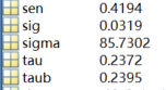
求一个序列的趋势,首先把x和y合成n×2的ts矩阵
再应用ktaub代码,可以把ktaub.m放到当前目录,推荐加到环境变量
tb = csvread('data.csv', 1, 0);
[m, n] = size(tb);
ts1 = [1:m]';
ts2 = tb(:,2);
ts = [ts1,ts2];
[taub tau h sig Z S sigma sen] = ktaub(ts, 0.05)
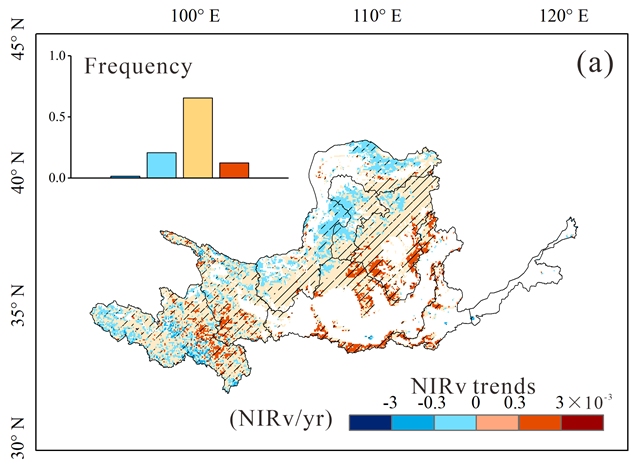
% 利用Mann-Kendall方法计算NDVI的年际趋势
% load('H:\MODIS_WUE\NH_20171009\gimms3gv1\ndvi_season.mat', 'ndvi_spring')
% load('H:\MODIS_WUE\NH_20171009\boundary\mask_pft.mat', 'mask_pft')
[m,n,z] = size(GPP_modfix);
slope_GPPmodfix = nan(m,n);
p_GPPmodfix = nan(m,n);
for i = 1:m
    for j = 1:n
%         if isnan(mask_pft(i,j))
%             continue
%         end
        ts1 = [1:z]';
        ts2 = permute(GPP_modfix(i,j,:),[3 1 2]);
        k = find(~isnan(ts2));
        ts1 = ts1(k);
        ts2 = ts2(k);
        ts = [ts1,ts2];
        if ~isnan(ts)
            [taub tau h sig Z S sigma sen] = ktaub(ts,0.05);
            slope_GPPmodfix(i,j) = sen;
            p_GPPmodfix(i,j) = sig;
        end
    end
end
完整代码见文末
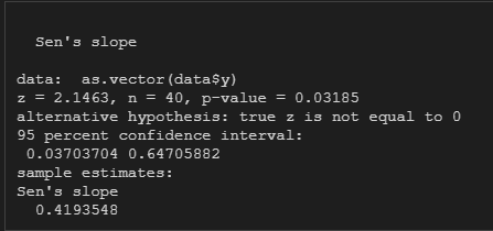
R是利用trend包中的sens.slope方法,同样这个包还提供了检验。
library(tidyverse)
library(trend)
df = read.csv('D:/OneDrive/GitHub/statistic/Mann-Kendall/data.csv')
y <- as.numeric(unlist(df['data']))
sens.slope(as.vector(data$y), conf.level = 0.95)
VPA中的方差分解是分析影响内生变量的结构冲击的贡献度。
原理是自变量变化会对因变量产生贡献,利用方差分解分析VPA(Variance Partitioning Analysis)可以计算各自变量的贡献程度。
在地球环境科学的实际应用中,可以基于VPA结果得出不同类型的环境因素(如何气候、土壤性质以及植物)对生物群落组成(如植被丰度,微生物群落)的解释程度。
在 R 中进行方差分解同样离不开vegan包,主要依赖两个功能:
- 变量筛选
ordistep - 方差分解
varpart
在进行任何多变量的分析,必须考虑变量之间存在的相关性。除了主成分分析,可以用RDA分析
冗余分析(redundancy analysis,RDA)是一种回归分析结合主成分分析的排序方法,也是多响应变量(multiresponse)回归分析的拓展。从概念上讲,RDA是响应变量矩阵与解释变量之间多元多重线性回归的拟合值矩阵的PCA分析。
代码如下:
library(vegan)
library(tidyverse)
data(mite)
data(mite.env)
data(mite.pcnm)
rda_full <- rda(mite~., data = cbind(mite.pcnm, mite.env))
rda_null <- rda(mite~1, data = cbind(mite.pcnm, mite.env))

rda_back <- ordistep(rda_full, direction = 'backward',trace = 0)

# forward selection
rda_frwd <- ordistep(rda_null, formula(rda_full), direction = 'forward',trace = 0)

# bothward selection
rda_both <- ordistep(rda_null, formula(rda_full), direction = 'both',trace = 0)
关于ordistep的说明文档可以见R的参考文档:https://rdrr.io/rforge/vegan/man/ordistep.html
约束排序方法 ( cca, rda, capscale) 的自动逐步模型构建。该函数ordistep是仿照的step,可以使用排列测试进行前向、后向和逐步模型选择。对于由或创建的排序对象,函数ordiR2step仅对调整后的 R2和 P 值执行正向模型选择。
总体上,根据一系列“黑盒”操作,选择出主要的变量。
结果如图,根据rda_both结果:

在mite.env因素中选择了WatrCont因子,在mite.pcnm因素中选择了V2和V6因子
在进行VPA时,首先就要对这些环境因子进行一个分类,然后在约束其它类环境因子的情况下,对某一类环境因子进行排序分析,这种分析也成为偏分析,即partialRDA。
在对每一类环境因子均进行偏分析之后,即可计算出每一个环境因子单独以及不同环境因子相互作用分别对生物群落变化的贡献。
首先是两类的情况,书接上文,把环境因子分为mite.env和mite.pcnm两类,即环境因子和空间相邻因子
df_env <- mite.env %>% select(WatrCont)
df_pcnm <- mite.pcnm %>% select(V2, V6)

# Perform variation partitioning analysis, the first variable is the community matrix
# the second and third variables are climate variable set and soil property variable set
vpt <- varpart(mite, df_env, df_pcnm)
格式是varpart(因变量,第一类因子,第二类因子)
结果如图:

a为X1也就是环境因素单独对群落变化的贡献。
b为X2也就是空间相邻因素对群落变化的贡献。
c为X1和X2的相互作用对群落变化的贡献,这里是0
d为X1和X2无法解释的群落变化。
接下来绘韦恩图
plot(vpt, bg = 2:5, Xnames = c('env', 'pcnm'))

环境因素解释了20%
接下来计算显著性
formula_env <- formula(mite ~ WatrCont + Condition(V2) + Condition(V6))
formula_pcnm <- formula(mite ~ Condition(WatrCont) + V2 + V6)

anova(rda(formula_env, data = cbind(mite.pcnm, mite.env)))
anova(rda(formula_pcnm, data = cbind(mite.pcnm, mite.env)))

单独计算环境因素和空间相邻因素的显著性,结果环境因素非常显著(p < 0.01),空间相邻因素比较显著 (p < 0.05)
mod <- varpart(mite, ~ SubsDens + WatrCont, ~ Substrate + Shrub + Topo,
               mite.pcnm, data=mite.env, transfo="hel")
plot(mod, bg=2:4, Xnames = c('SubsDens + WatrCont', 'Substrate + Shrub + Topo', 'pcnm'))
