UNIFORM B-SPLINE CERES

A B-spline optimization library to optimize uniform B-spline with ceres.

Usage

Fitting a 1D spline to std::exp function.

In this example we build and solve a ceres problem of fitting a 1D spline to a test function. The test function will be $f(x) = \exp(2x)$. We use a 1D spline with degree of three.

using Spline = ubs::UniformBSpline<double, 3, double, double, std::vector<double>>;

We begin with defining the residual function:

class ExponentialResidual {
public:
    explicit ExponentialResidual(const ubs::UniformBSplineCeresEvaluator<Spline>& splineEvaluator, double measurement)
            : splineEvaluator_(splineEvaluator), measurement_{measurement} {
    }

    template <typename T>
    bool operator()(const T* c0, const T* c1, const T* c2, const T* c3, T* residual) const {
        splineEvaluator_.evaluate(c0, c1, c2, c3, residual);
        *residual -= T(measurement_);
        return true;
    }

private:
    ubs::UniformBSplineCeresEvaluator<Spline> splineEvaluator_;
    double measurement_;
};

Our parameters of the cost functor are the control points. As we use a spline with degree of three, the order is four and we need four control points to evaluate the spline. Those are the input parameters. Using the control points we evaluate the spline using the splineEvaluator. The result will be stored in residual. The residual is the distance between the spline value and the measurement.

Now we need to create the ceres problem. At first the number of control points needs to be specified. In this example we are using 20 control points all set to zero.

    std::vector<double> controlPoints(20, 0.0);
    Spline spline(controlPoints);
    ubs::UniformBSplineCeres<Spline> splineCeres(spline);

The next step is to setup the problem.

    std::vector<double*> parameterPointers(splineCeres.getNumPointParameterPointers());
    ceres::Problem problem;

    for (int i = 0; i < numMeasurements; ++i) {
        const double posX = double(i) / double(numMeasurements);
        const double posY = std::exp(posX * 2.0);

        const auto data = splineCeres.getPointData(posX);
        splineCeres.fillParameterPointers(data, parameterPointers.begin(), parameterPointers.end());
        ubs::UniformBSplineCeresEvaluator<Spline> evaluator = splineCeres.getEvaluator(data);

        auto* costFunctor = new ceres::AutoDiffCostFunction<ExponentialResidual, 1, 1, 1, 1, 1>(
            new ExponentialResidual(evaluator, posY));

        problem.AddResidualBlock(costFunctor, nullptr, parameterPointers);
    }

We generate a residual for each measurement. What we would like to do is to evaluate the spline in the residual. This is where splineCeres helps. First, one need the evaluation data at a single point by calling getPointData(). The returned data is used to retrieve the parameter pointers and the evaluator. The parameter pointers are passed to ceres during the call to AddResidualBlock. The spline evaluator is passed to the residual and used to calculate the spline value during optimization. The number of parameter blocks is the order of the spline, each of which has one dimension. So the AutoDiffCostFunction parameter block sizes are 1 for the output residual and 4 times 1 for the control points.

The last step is solving the problem:

    ceres::Solver::Options options;
    options.minimizer_progress_to_stdout = true;
    ceres::Solver::Summary summary;
    ceres::Solve(options, &problem, &summary);
    std::cout << summary.FullReport() << std::endl;

To see the full example see evaluator_example.cpp.

Optimizing a spline with variable evaluation position

In the last example the evaluation point of the spline has to be known before and was fixed during solving the problem. In this section we well see an example on how a problem can be solved, if the evaluation point is not fixed during optimization.

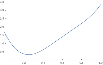
As an example we search for a minimum of a 1D -> 1D spline while keeping the control points fixed. The spline will look like this:

First we need to define the type of our spline.

template <typename T>
using Spline = ubs::UniformBSpline<T, 3, T, T, std::vector<T>>;

This is a 1D -> 1D spline of order of 3 where the control points are stored in a std::vector. The spline is templated as we need to use it for building the problem, where T is double, and in an autodiff cost function, where T is ceres::Jet.

Next we define our residual function:

class SplineMinimumResidual {
public:
    explicit SplineMinimumResidual(const ubs::UniformBSplineCeresGenerator<Spline>& generator, int numControlPoints)
            : generator_(generator), numControlPoints_(numControlPoints) {
    }

    template <typename T>
    bool operator()(const T* const* paramPointers, T* residual) const {
        const T* const* controlPoints = paramPointers;
        const T& pos = *(paramPointers[numControlPoints_]);

        auto spline = generator_.generate(controlPoints);
        residual[0] = spline.evaluate(pos);
        residual[1] = spline.derivative(pos, 1);
        return true;
    }

private:
    ubs::UniformBSplineCeresGenerator<Spline> generator_;
    int numControlPoints_;
};

The constructor takes the number of control points and a spline generator. A spline generator is used to generate an auto differentiable spline based on the control points in the cost function. To calculate the residual we first extract the control points parameter pointers and the evaluation point. Then a spline is generated using the generator. The generator returns a ubs::UniformBSpline object with a value type of type T. Now the spline can be used as it would be a regular spline. We evaluate two residuals, the value and its first derivative of the spline at pos and assign them to the residual vector. This function is minimal, when the spline value is minimal and the derivative is zero.

The next step is to initialize a spline, create the ceres problem and solve it.

So first let us initialize a spline and ceres spline object with seven control points:

    std::vector<double> controlPoints{6.0, 1.0, 0.0, 1.0, 2.0, 3.0, 6.0};
    Spline<double> spline(controlPoints);
    ubs::UniformBSplineCeres<Spline<double>> splineCeres(spline);

    double t = 0.8;

t is the spline evaluation point which we would like to optimize. The initial value is set to 0.8. Now need to get the parameter pointers and spline generator to build our residual. At first we need to get a range data object

    const auto data = splineCeres.getRangeData(0.0, 1.0);

Here our range is $[0.0, 1.0]$ as we would like to evaluate the spline in that range. The range highly influences the sparsity of the problem. If the range is the full range of the spline, all control points are depending on it. On the other hand, if the range is almost zero, the number of depending control points is only the order of the spline.

Now lets build the parameter vector using the range data:

    const int numControlPoints = splineCeres.getNumRangeParameterPointers(data);
    std::vector<double*> parameterPointers(numControlPoints + 1);

    splineCeres.fillParameterPointers(data, parameterPointers.begin(), parameterPointers.begin() + numControlPoints);
    parameterPointers.back() = &t;

We determine the number of control points. The total number of parameters for the cost functor is the number of control points plus one because of the spline evaluation position t. Then we fill the first part of the parameter vector with the control points and the last pointer with evaluation point.

Now lets create our cost function:

    ubs::UniformBSplineCeresGenerator<Spline> generator = splineCeres.getGenerator<Spline>(data);

    auto costFunction = std::make_unique<ceres::DynamicAutoDiffCostFunction<SplineMinimumResidual>>(
        new SplineMinimumResidual(generator, numControlPoints));

    for (int i = 0; i < numControlPoints; ++i) {
        costFunction->AddParameterBlock(1);
    }
    costFunction->AddParameterBlock(1);
    costFunction->SetNumResiduals(2);

In order to get the spline generator needed for construct our residual, we call ubs::UniformBSplineCeres::getGenerator. The UniformBSplineCeres::getGenerator function takes the range data and a template template parameter of the spline. The passed spline must accept one template parameter value type. This is needed to create the correct spline during optimization, as it is not yet known.

Then the residual is generator and the parameter pointer dimensions are set. Each control point has a dimensionality of 1 and the evaluation point also has a dimension of 1. As we are using the spline value and its first derivative as residual, the residual dimension is 2.

Now lets setup the problem:

    ceres::Problem problem;
    problem.AddResidualBlock(costFunction.release(), nullptr, parameterPointers);

As the spline can only be evaluated in the interval $[0.0, 1.0]$, we set a lower and upper bound accordingly:

    problem.SetParameterLowerBound(&t, 0, 0.0);
    problem.SetParameterUpperBound(&t, 0, 1.0);

Also we would like to fix all control points. This can be done by using the ubs::UniformBSpline::getControlPointsContainer. The container provides a method of iteration over all control points.

    spline.getControlPointsContainer().forEach([&](double& c) { problem.SetParameterBlockConstant(&c); });

As a last step the problem is solved.

    ceres::Solver::Options options;
    options.minimizer_progress_to_stdout = true;
    options.parameter_tolerance = 1e-15;
    options.gradient_tolerance = 1e-15;
    options.function_tolerance = 1e-15;

    ceres::Solver::Summary summary;
    ceres::Solve(options, &problem, &summary);
    std::cout << summary.FullReport() << std::endl;

Using the control points above the minimum will be 0.25.

To see the full example see generator_example.cpp.

Smoothing / Regularization

There are different ways of expressing smoothness of a function. One way is a integral over the absolute function or its derivative:

$$s_i = \int_0^1 \lVert f_i^{(n)}(\mathbf{x}) \rVert^2 \mathbf{dx}$$

In the one dimensional case this expression can be can efficiently integrated in a least-squares problem, as one can exactly

$$s_i = \int_0^1 \lVert f_i^{(n)}(x) \rVert^2 dx = \sum_i^{N-o} \lVert s \mathbf{B}^{1/2} \mathbf{P}_{i:i+o} \rVert^2$$

This means the integral can be expressed as a sum of a matrix matrix product where $s \mathbf{B}^{1/2}$ can be precomputed and $\mathbf{P}_{i:i+o}$ are the control points from $i$ to $ i + o$ and $o$ is the order of the spline.

For the one-dimensional case the formula above can be used directly. The control points are lay out in a line.

Here the red dots are the control points and the black line is the one-dimensional spline which is used for smoothing.

In the two-dimensional case, such a integral can also be solved and efficiently integrated into an NLS problem.

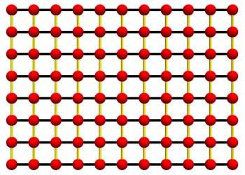
For higher order splines an approximation is implemented using the one-dimensional case. E.g. in the two-dimensional case the control points are lay out in a grid.

To smooth such a spline one create a one-dimensional spline in each grid direction (horizontal and vertical). Those splines are shown in black and yellow.

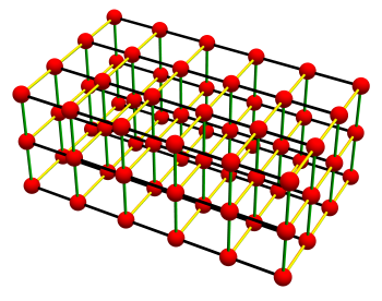
In the three-dimensional case the control points are organized in a three-dimensional grid. Here one-dimensional splines in each directions are build and used for smoothing (black, yellow and green lines).

To add the exact smoothing residuals to the ceres problem a call to UniformBSplineCeres::addSmoothnessResiduals is sufficient.

    const double weight = 1e-5;
    splineCeres.addSmoothnessResiduals<1>(problem, weight);

The first argument is the ceres problem to which the cost functions are added. The second one is the weight used to scale the smoothness. The higher the weight the smoother the function will be. The template parameter is the derivative of the function which is used for smoothing.

To add the grid based approximation one have to call UniformBSplineCeres::addSmoothnessResidualsGrid.

    splineCeres.addSmoothnessResidualsGrid<1>(problem, weight);