The partial discharge (PD) detection is of critical importance in the stability and continuity of power distribution operations. Although several feature engineering methods have been developed to refine and improve PD detection accuracy, they can be suboptimal due to several major issues: (i) failure in identifying fault-related pulses, (ii) the lack of inner-phase temporal representation, and (iii) multi-scale feature integration. The aim of this paper is to develop a Learning based Multiscale Feature Engineering (LMFE) framework for PD detection of each signal in a 3-phase power system, while addressing the above issues. The 3-phase measurements are first preprocessed to identify the pulses together with the surrounded waveforms. Next, our feature engineering is conducted to extract the global-scale features, i.e., phase level and measurement level aggregations of the pulse-level information, and the local-scale features focusing on waveforms and their inner-phase temporal information. A recurrent neural network (RNN) model is trained, and intermediate features are extracted from this trained RNN model. Furthermore, these multi-scale features are merged and fed into a classifier to distinguish the different patterns between faulty and non-faulty signals. Finally, our LMFE is evaluated by analyzing the VSB ENET dataset, which shows that LMFE outperforms existing approaches and provides the state-of-the-art solution in the PD detection.
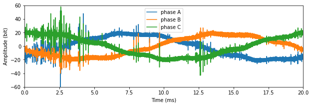
Examples of Three-phase Measurement Signals
Fig 1. Examples of (a) normal signals and (b) faulty signals in 3-phase measurements.
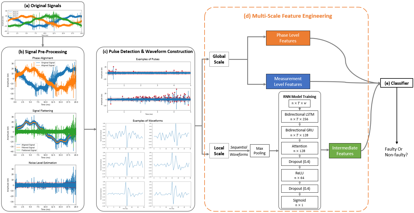 Fig 2. The workflow of proposed LMFE for PD detection: (a) original signals for one measurement; (b) signals preprocessing including phase alignment,
signal flattening, and noise estimation; (c) pulses & surrounded waveforms identification; (d) multi-scale feature engineering including (1) global-scale features based on both phase-level and measurement-level summary statistics of features extracted from pulses and waveforms, and (2) local-scale features extracted from a RNN model using the sequential waveforms as input; (e) final detection based on combinations of multi-scale features.
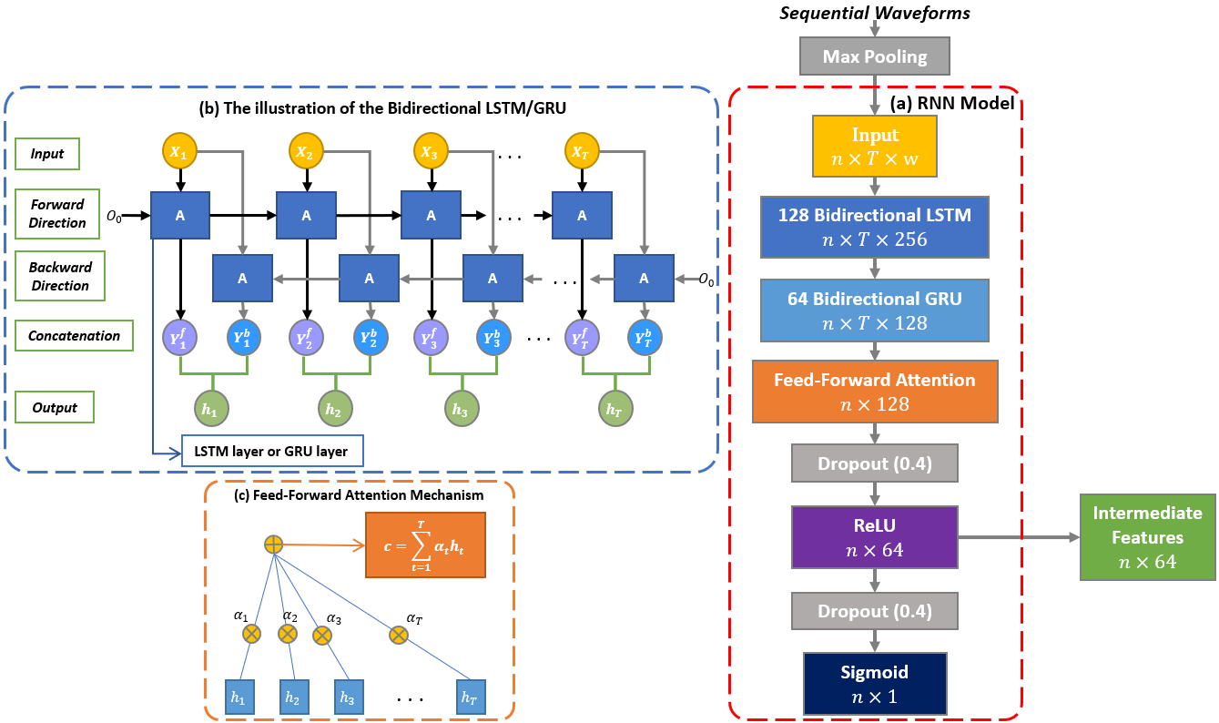
Details of the construction of local-scale features
Fig 3. Details of the construction of local-scale features: (a) the architecture of the RNN model; (b) the illustration of the bidirectional LSTM/GRU; (c) the illustration of feed-forward attention layer. Here T is the number of waveforms in each signal, w is the length of each waveform, and n is the number of signals.
run the following via the command:
python main_cmd.py -h
A list of detailed command-line options
usage: main_cmd.py [-h] [--data_dir DATA_DIR] [--input_dir INPUT_DIR]
       [--preprocessed] [--recalculate_peaks] [--nchunks NCHUNKS]
       [--NN_level NN_LEVEL] [--NN_model NN_MODEL]
       [--Dense_layers DENSE_LAYERS] [--NN_pretrained]
       [--classifier CLASSIFIER]
       [--classifier_level CLASSIFIER_LEVEL]
       [--num_iterations NUM_ITERATIONS]
       [--kfold_random_state KFOLD_RANDOM_STATE]
       [--num_folds NUM_FOLDS] [--feature_set FEATURE_SET]
       [--local_features] [--load_local_features] [--iter ITER]
       [--layer_idx LAYER_IDX] [--NN_batch_size NN_BATCH_SIZE]
       [--monitor MONITOR] [--dropout DROPOUT]
       [--regularizer REGULARIZER] [--loss_name LOSS_NAME]
       [--from_logits] [--kernel_size KERNEL_SIZE]
       [--n_epochs N_EPOCHS] [--pretrained] [--NN_only]
       [--units UNITS] [--predict] [--load_attention_weights]
       [--extract_attention_weights]

Choice of RNN model, classifier, training level and number of dense layers

optional arguments:
  -h, --help            show this help message and exit
  --data_dir DATA_DIR   the folder path for signal data
  --input_dir INPUT_DIR
      the folder path for the preprocessed data
  --preprocessed        if the preprocessing steps have done for waveform and
      global feature extraction
  --recalculate_peaks   whether to recalculate the peaks in the preprocessing
      step, only valid when preprocessed=False
  --nchunks NCHUNKS     number of chunks in waveforms, choose from
      100,160,200,400
  --NN_level NN_LEVEL   RNN training level
  --NN_model NN_MODEL   choose from LSTM and minimal_rnn, or TCN
  --Dense_layers DENSE_LAYERS
      number of dense lyaers in RNN, choose from 1,2,3
  --NN_pretrained       if the RNN model is well-trained
  --classifier CLASSIFIER
      classifier, choose from LightGBM, XGboost,
      random_forest
  --classifier_level CLASSIFIER_LEVEL
      Classification training level
  --num_iterations NUM_ITERATIONS
      number of iterations for classifier
  --kfold_random_state KFOLD_RANDOM_STATE
      random seeds for splitting the k-folds
  --num_folds NUM_FOLDS
      number of folds for cross-validation
  --feature_set FEATURE_SET
      features to be input to classifier, choose from
      global, phase, measurement
  --local_features      include the intermediate features or not
  --load_local_features
      whether to load the intermediate features or extract
      from the netwrok
  --iter ITER           iteration index, ranging from 0 to num_iterations-1
  --layer_idx LAYER_IDX
      layer_idx to extract the intermediate features
  --NN_batch_size NN_BATCH_SIZE
      batch size for RNN training
  --monitor MONITOR     monitor the improvement of val_loss or
      val_matthews_correlation_2 (i.e., 1-mcc) in the RNN
      model
  --dropout DROPOUT     dropout ratio in the RNN model
  --regularizer REGULARIZER
      use l1 or l2 penalty in the RNN model
  --loss_name LOSS_NAME
      loss function used in the RNN model, choose from bce,
      weighted_bce, focal
  --from_logits         training from logits or not
  --kernel_size KERNEL_SIZE
      kernel size of Conv1D in TCN
  --n_epochs N_EPOCHS   number of epochs for NN model
  --pretrained          if classifier is trained well
  --NN_only             if get results from the network only
  --units UNITS         hidden layers in MLP classifier
  --predict             if the model is evaluated by prediction performance
  --load_attention_weights
      whether to load the attention weights or recalculate
      it
  --extract_attention_weights
      whether to extract the attention weights for analysis,
      only valid when load_attention_weights=False
- SIGNAL_DATA_FOLDER
- PREPROCESSED_DATA_FOLDER
- global_features.csv
- kmeans.dat
- kmeans_A.dat
- kmeans_B.dat
- kmeans_C.dat
- all_chunk_waves_*chunks.dat
- RESULTS_FOLDER
- models
- global_scale
- RNN_weights
- models
The settings:
chunk size = 200, NN_level = 'signal', NN_model = 'LSTM', Dense_layer = 2, classifier = 'XGboost', classifier_level = 'measurement', num_iterations = 25, num_folds = 5, feature_set = 'global', layer_idx = 5, monitor = 'val_loss', loss_name = 'weighted_bce', from_logits = True,
(i) Training from scratch
python main_cmd.py --data_dir SIGNAL_DATA_FOLDER --input_dir PREPROCESSED_DATA_FOLDER --local_features
                   --nchunks 200 --NN_level signal --NN_model LSTM --Dense_layers 2 --classifier XGboost
                   --classifier_level measurement --num_iterations 25 --num_folds 5 --features_set global
                   --layer_idx 5 --dropout 0.4 --regularizer l2 --loss_name weighted_bce --from_logits
                   --predict
(ii) If the preprocessing steps are done, the neural network is trained well, and the local-scale features have been extracted
Add the following arguments
--preprocessed --NN_pretrained --load_local_features (iii)To further extract the attention weights for analysis
python main_cmd.py --data_dir SIGNAL_DATA_FOLDER --input_dir PREPROCESSED_DATA_FOLDER --NN_only
                   --nchunks 200 --NN_level signal --NN_model LSTM --Dense_layers 2
                   --num_iterations 25 --num_folds 5 --dropout 0.4 --regularizer l2
                   --loss_name weighted_bce --from_logits --preprocessed --NN_pretrained
--extract_attention_weightsAssume that the preprocessing steps have been done
python main_cmd.py --data_dir SIGNAL_DATA_FOLDER --input_dir PREPROCESSED_DATA_FOLDER --NN_only
                   --nchunks 200 --NN_level signal --NN_model LSTM --Dense_layers 2
                   --num_iterations 25 --num_folds 5 --dropout 0.4 --regularizer l2
--loss_name weighted_bce --from_logits --predict (i) All the global-scale features
python main_cmd.py --data_dir SIGNAL_DATA_FOLDER --input_dir PREPROCESSED_DATA_FOLDER
                   --nchunks 200 --NN_level signal --NN_model LSTM --Dense_layers 2 --classifier XGboost
                   --classifier_level measurement --num_iterations 25 --num_folds 5 --features_set global
                   --layer_idx 5 --dropout 0.4 --regularizer l2 --loss_name weighted_bce --from_logits
                   --predict
(ii) Only the phase-level features
--feature_set phase_level
(iii) Only the measurement-level features
--feature_set measurement_level
python visualization_preprocess.py
python results_analysis.py
Model_performance.ipynb presents the performance comparison.
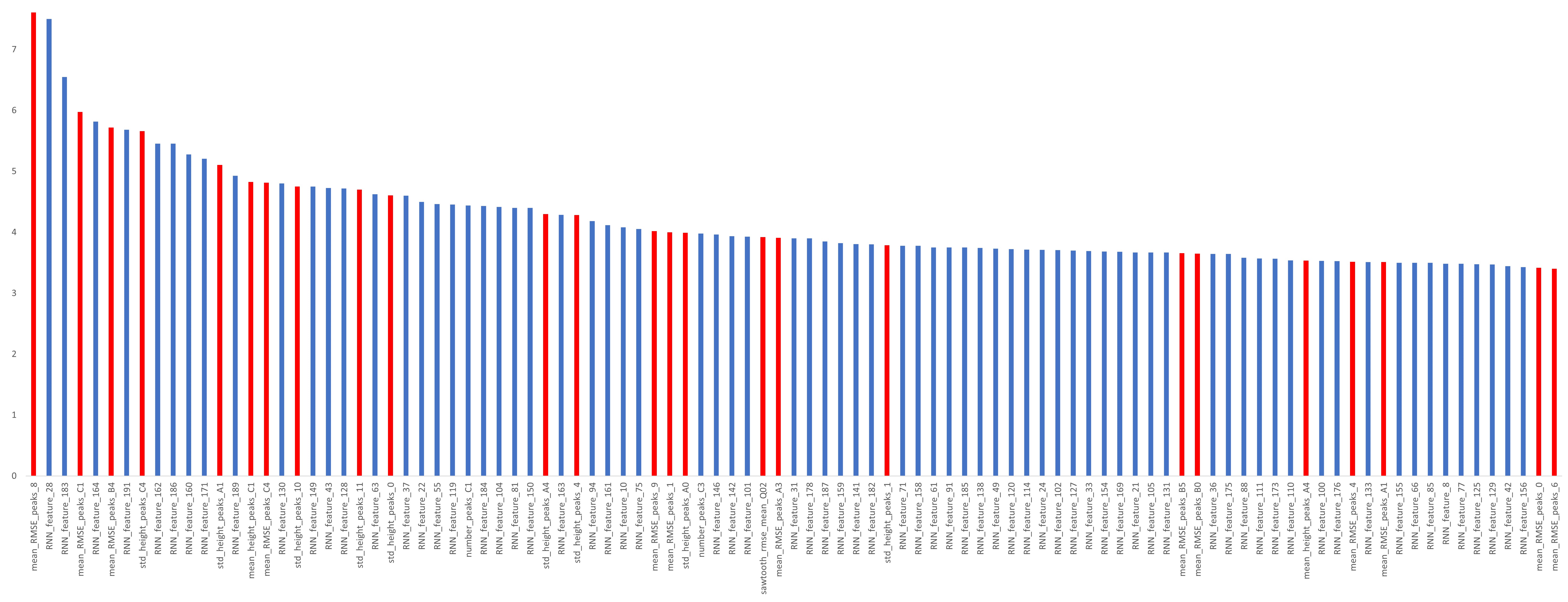
The top 100 important features
Fig 4. The top 100 important features sorted by the logarithm-scale importance gain. The local-scale features are highlighted in blue, while the global-scale features are indicated in red.
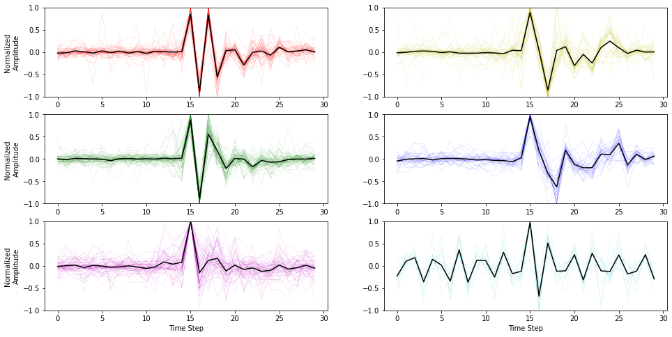
Cluster centroids for representative waveforms from faulty signals
Fig 5. The centroids for the waveform with the largest weights of different clusters for all faulty signals when k = 6.
https://www.kaggle.com/competitions/vsb-power-line-fault-detection
-
The keras implementation of MinimalRNN is from https://github.com/titu1994/keras-minimal-rnn.
-
The code for preprocessing steps and global-scale feature extraction is from Kunjin Chen @yalikjc,
Reference: Chen, K., Vantuch, T., Zhang, Y., Hu, J., & He, J. (2020). Fault detection for covered conductors with high-frequency voltage signals: From local patterns to global features. IEEE Transactions on Smart Grid, 12(2), 1602-1614.

