In this project, we try to build an advanced lane detection system to augment video output with detected road lane, road-radius curvature and road-centre offset.
A clear working of the project is provided in the docs folder. To access the docs, please install draw.io plugin for Visual Studio Code by doing the following:
- open vs-code
- press ctrl+p
- ext install hediet.vscode-drawio
Camera Calibration Image distortion occurs when cameras look at objects that have 3D features in the real world and want to transform them into 2D planes in the image. This transformation is not efficient and would bring a lot of distortion to the picture. This distortion changes the shape and size of the object in this transformation. So, the first step in analyzing the image distortion level is the pre-processing step.
This step has a significant effect on the performance of lane detection because distorted images show the lane of the image in some parts curvy, keep out the detection application from reality and make an image look tilted so that some objects appear farther away or closer than they are in fact. Camera Calibration maps 3D points 2D points one. This can be done with images with grid patterns such as a chessboard. This process uses multiple photos of chessboards from different distances and angles. The images are put as input and return the camera calibration values. We use this value matrix with the original images of datasets to make them unsorted images.
Steps:
- undistort the images coming from camera, thus improving the quality of geometrical measurement.
- estimate the spatial resolution of pixels per meter in both x and y directions
For this project, the calibration pipeline is implemented in function calibrate implemented in file calibrate.py. The procedure follows these steps:
-
The procedures start by preparing "object points", which will be the
(x, y, z)coordinates of the chessboard corners in the world. Here I am assuming the chessboard is fixed on the (x, y) plane at z=0. Also, I am assuming that the size of the chessboard pattern is the same for all images, so the object points will be the same for each calibration image. -
Then, the calibration images are sequentially loaded, converted to grayscale and chessboard pattern is looked for using
cv2.findChessboardCorners. When the pattern is found, the positions of the corners get refined further to sub-pixel accuracy usingcv2.cornerSubPix. That improves the accuracy of the calibration. Corner coordinates get appended to the list containing all the image points, while prepared "object points" gets appended to the list containing all the object points. -
The distortion coefficients and camera matrix are computed using
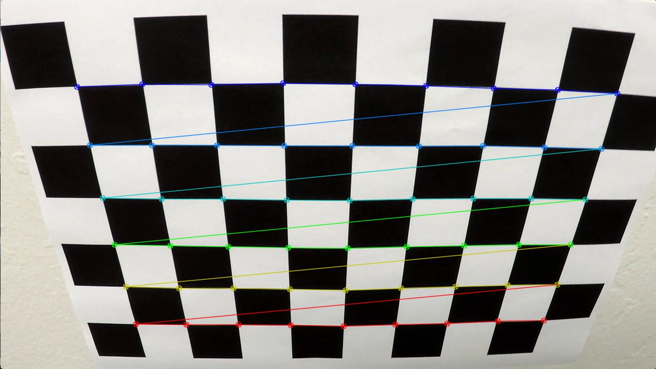
cv2.calibrateCamera()function, where image and object points are passed as inputs. It is important to check if the result is satisfactory, since calibration is a nonlinear numerical procedure, so it might yield suboptimal results. To do so calibration images are read once again and undistortion is applied to them. The undistorted images are shown in order to visually check if the distortion has been corrected. Once the data has been checked the parameters are is pickled saved to file. One sample of the input image, image with chessboard corners and the undistorted image is shown:
| Original image | Chessboard corners | Undistorted image |
|---|---|---|
 |
 |
 |
The camera matrix encompases the pinhole camera model in it. It gives the relationship between the coordinates of the points relative to the camera in 3D space and position of that point on the image in pixels. If X, Y and Z are coordinates of the point in 3D space, its position on image (u and v) in pixels is calculated using:
where M is camera matrix and s is scalar different from zero. This equation will be used later on.
| Pinhole camera model |
|---|
 |
Install all requirements by
pip3 install -r requirements.txt
Next step is to find the projective transform so the original images can be warped so that it looks like the camera is placed directly above the road. OOne approach is to hand tune the source and destination points, which are required to compute the transformation matrix. On the other hand, the script that does that for us can be created based on linear perspective geometry. Let's look at the perspective geometry on the renaissance painting "Architectural Veduta" by Italian painter Francesco di Giorgio Martini. It is easy to note that all lines meet at a single point called vanishing point. The second thing to note is that the square floor tiles centered horizontally in the image, appear as trapezoids with horizontal top and bottom edges and side edges radiating from the vanishing point.
| Architectural Veduta |
|---|
 |
Our goal is to achieve exactly opposite, to transform a trapezoidal patch of the road in front of the car to a rectangular image of the road. To do so, the trapezoid needs to be defined as previously noted, horizontal top and bottom centered with respect to a vanishing point, sides radiating from the vanishing point. Of course, to define that, the first task is to find the vanishing point.
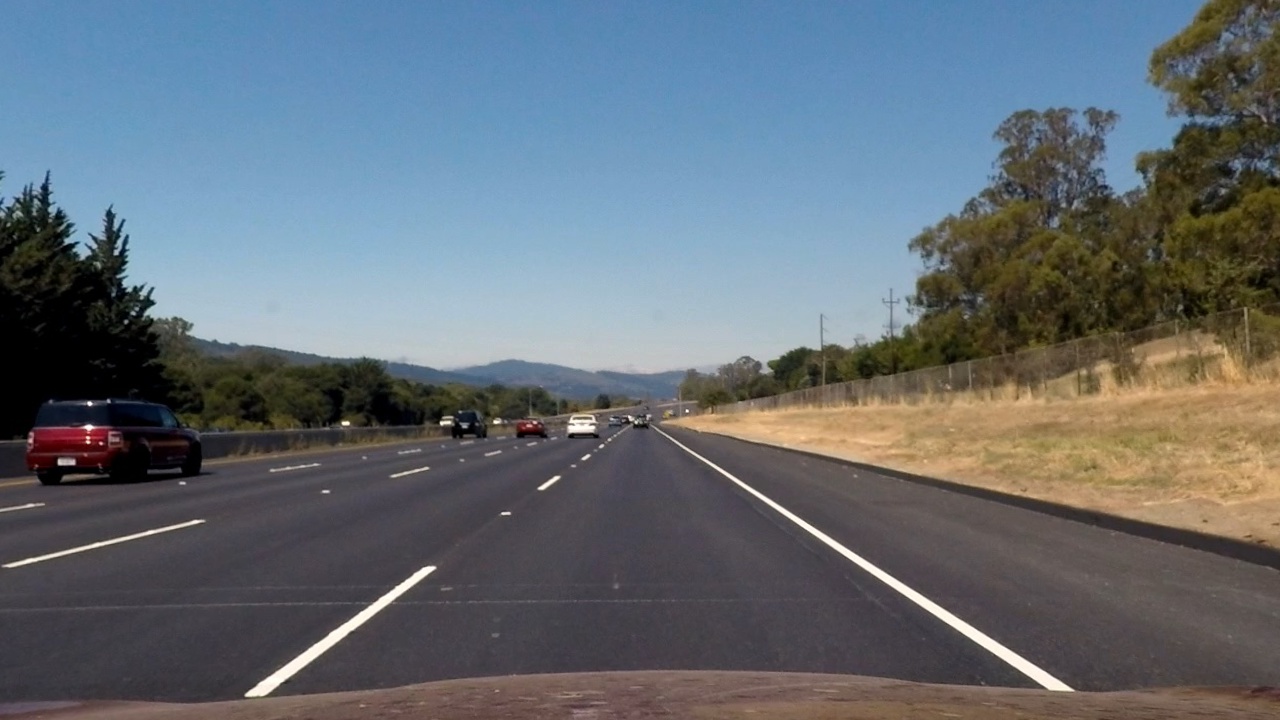
The vanishing point is the place where all parallel lines meet, so to find it we will be using images with straight lines straight_lines1.jpg, straight_lines2.jpg. First, the images are undistorted, the Canny filter is applied and most prominent lines are identified using cv2.HoughLinesP. These images show how the pipeline works:
| Undistorted image | Edges | Image with lines |
|---|---|---|
 |
 |
 |
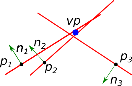
All detected lines are added to a list. The vanishing point is at the intersection of all the lines from the list. Unfortunately, when more than two lines are present, the unique intersecting point might not exist. To overcome that the vanishing point is selected as the point whose total squared distance from all the lines is minimal, thus optimization procedure will be employed. Each line found by the Hough lines can be represented by the point on it pi and unit normal to it ni. Coordinate of the vanishing point is vp. So the total squared distance (and a cost function to be minimized is):
To find the minimum the cost function is differentiated with respect to the vp. After some derivation the following is obtained:
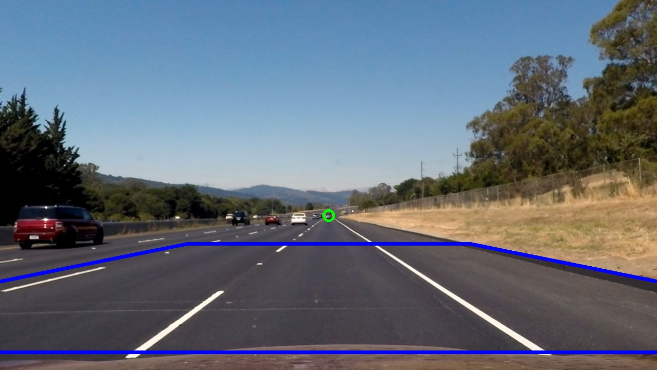
Once the vanishing point is found, the top and bottom are defined manually and the trapezoid edges can be calculated. The corners of the trapezoid are used as a source points, while destination points are four corners of the new image. The size of the warped image is defined in file settings.py. After that, the matrix that defines the perspective transform is calculated using cv2.getPerspectiveTransform(). The procedure that implements the calculation of homography matrix of the perspective transform is implemented at the beginning of the python script find_perspective_transform.py (lines 9 - 67). Images that illustrate the procedure follow. Please note that bottom points of the trapezoid are outside of the image, what is the reason for black triangles shown in the warped image.
| Finding VP with multiple lines | Trapezoid and vanishing point | Warped image |
|---|---|---|
 |
 |
 |
The obtained source and destination points are:
| Source | Destination |
|---|---|
| 375, 480 | 0, 0 |
| 905, 480 | 500, 0 |
| 1811, 685 | 500, 600 |
| -531, 685 | 0, 600 |
The selected range is quite big, but that had to be done in order to be able to find the lanes on the harder challenge video. In that video, the bends are much sharper than on the highway and might easily veer outside of the trapezoid causing the whole pipeline to fail.
Once again, lets just reflect on what is the matrix returned by the cv2.getPerspectiveTransform(). It tells how the perspective transformation is going to be performed and where the pixel from original image with the coordinates (u, v) is going to move after the transformation. The destination of that pixel on the warped image would be the point with the coordinates (uw, vw). The new position is calculated using::
where H is homography matrix returned as a result of cv2.getPerspectiveTransform() and s is scalar different from zero.
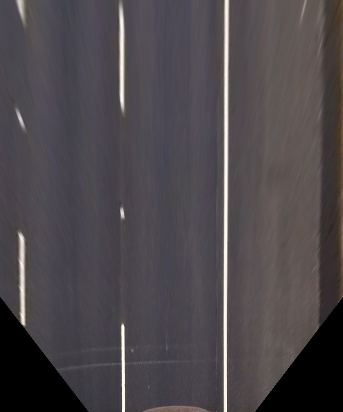
##Estimating pixel resolution Next important step is to estimate resolution in pixels per meter of the warped image. It also can be done by hand, but as previously we'll create a script that does that for us. In the course materials, it was stated that width of the lane is no less than 12 feet. In order to estimate the resolution in pixels per meter, the images with the straight lines will be used. They will be unwarped and the distance between the lines will be measured. The lower of two distances will be assumed to be 12 feet or 3.6576 meters.
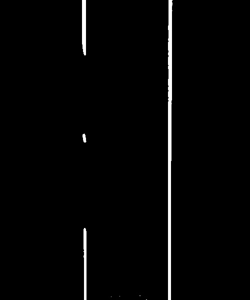
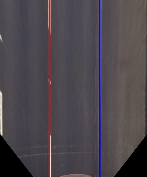
To start, the images with the straight lines would be unwarped and color would be converted to HLS space. To find the lanes the threshold would be applied to the luminesence component. Also, only some region of interest is taken into account. Since lines were straight heading towards the vanishing point, after the warping they will be vertical. The centroids of the blobs on left and right images would be calculated using image moments and function cv2.moments(). Since the lane lines are vertical the width of the lane in pixels is the difference between the x coordinates of two centroids. That allows for the calculation of the width in pixels and then resolution in x direction. This procedure is implemented between line 71 and
91 of the script find_perspective_transform.py. The images that illustrate the procedure are shown below.
| Warped image with parallel lane lines | Thresholded luminesence | Lane with lines identified |
|---|---|---|
 |
 |
 |
That is how to find resolution in x direction, but for finding resolution in y there is no such trick. Since nothing was estimated manually neither this will be. The camera matrix obtained by calibrations holds some relative information about resolutions in x and y direction. We can try to exploit that. To find resolution in y direction we have to do some more math.
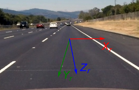
Lets say, we have a coordinate frame attached to the road, as shown on image below. It is easy to see that transformation of the coordinates represented in the coordinate frame of the road to the coordinate frame of the warped image, consists of scaling and shifted. Scale in x direction corresponds to the number of pixel per meter in x direction. Same holds for y. In mathemathical form that can be written as:
| Road frame as seen by camera | Road frame on warped image |
|---|---|
 |
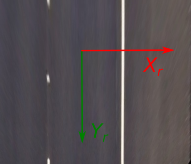 |
The same thing can be calculated from the other side. Lets say that position and of the road coordinate frame in camera coordinate frame is given with rotation matrix R=[r1 r2 r3] and translation vector t. One important property that is going to be exploited is that matrix R is orthogonal, meaning that each of the rows r1, r2, r3 has the length of 1. Now since we know that, the pixel on the image that corresponds to the point with coordinates Xr, Yr and Zr is calculated by:
Since the road is planar, the Zr=0. Now we apply the perspective transform and get:
Since it has to hold for every point we can conclude that:Where h1, h2, h3 are columns of matrix (HM)-1. Since the length of vectors r1 and r2 is one, we can calculate scalar s and finally ry:
The rather simple equation is obtained at the end, but it took us a while to get there. This calculation is implemented in lines 91 and 92 of script find_perspective_transform.py. The final result is:
| pix/meter in x direction | pix/meter in y direction |
|---|---|
| 46.567 | 33.0652548749 |
The pipeline is implemented in the class LaneFinder that does the lane finding and it is written in the file lane_finder.py. This class has two instances of subclass LaneLineFinder which is used to find a single line. The parts of the pipeline that have to be performed once (masking, calculating curvature, drawing an overlay etc...) on a whole image are encapsulated in the LaneFinder. The parts that have to be performed twice (fitting the line on a binary image), once for each line is encapsulated in LaneLineFinder. For easier explanation first, the functionality used for the single images will be explained. The pipeline for the video is almost the same, while some additional filtering is included.
The pipeline for single images goes through several steps. Let us see how initial image looks:
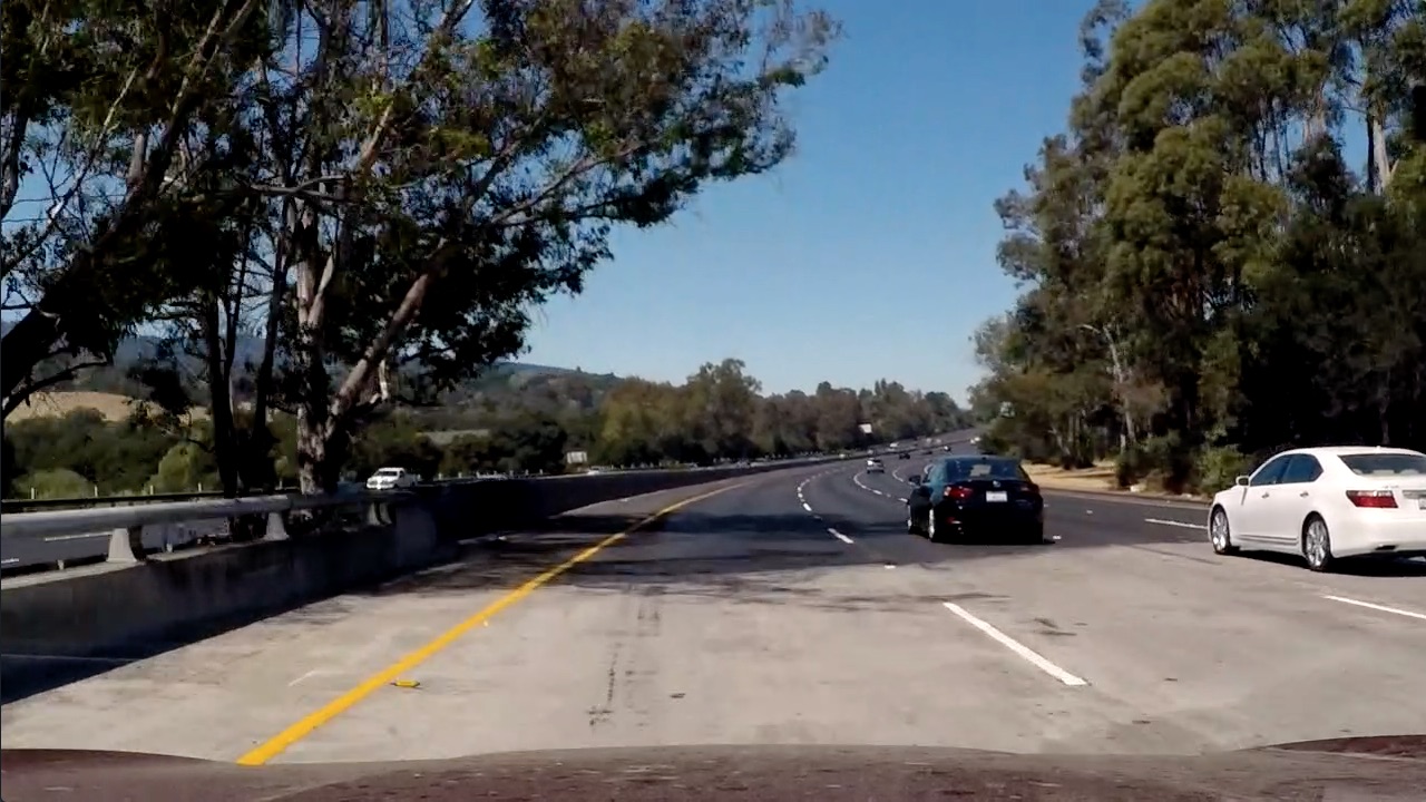
####1. Image undistortion, warping and color space conversion.
The image gets undistorted first, then the perspective transformation is applied to the undistorted image. After that, the images is converted into HLS and LAB color space. L channels of both HLS and LAB channels will be used to track the bright regions of the image, while B channel is used to track the yellow lines on the image. Also, some filtering is performed to reduce the noise, cv2.medianBlur() is used since it maintains the edges. Also for the use of the harder challenge video, the greenish areas are unmasked. Part of the code that performs this is from line 187 to 220. The undistorted and warped images are:
| Undistorted original image | Warped undistorted image |
|---|---|
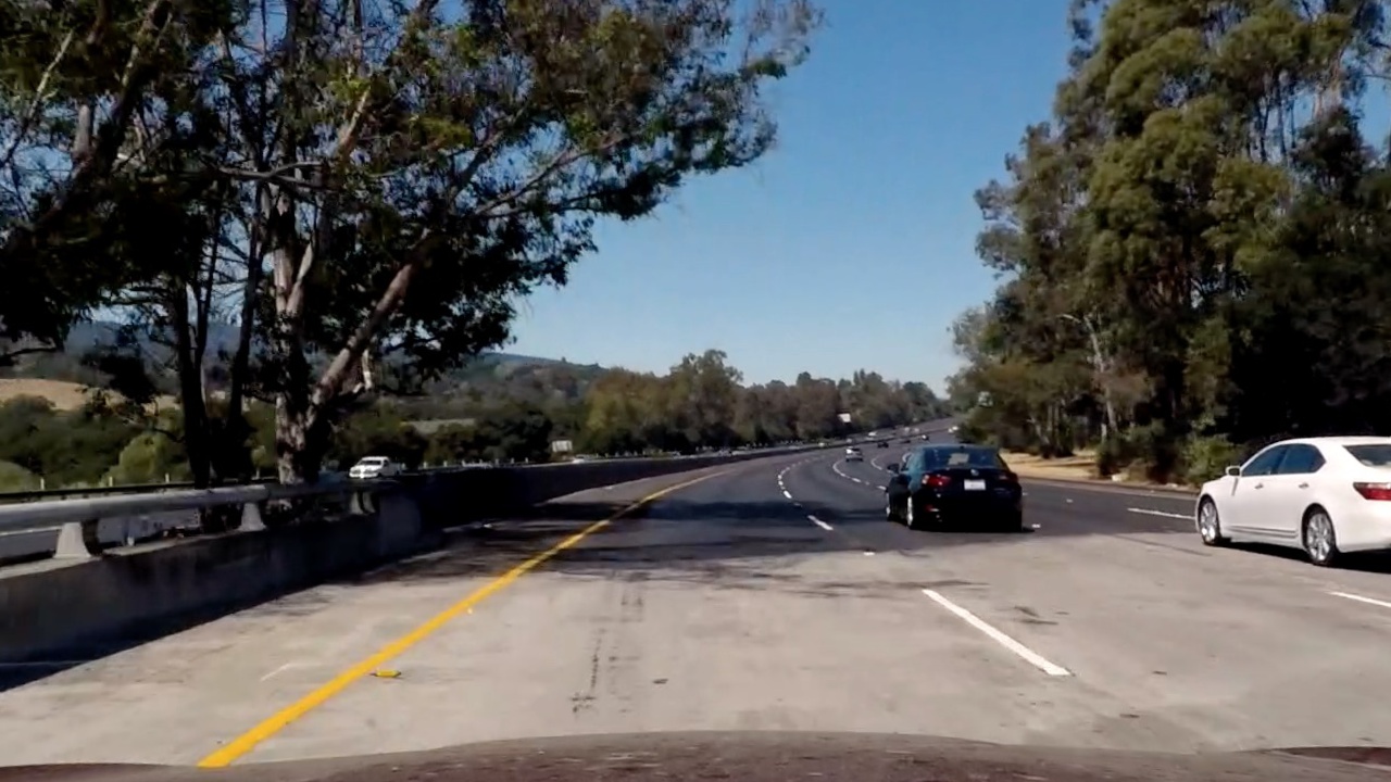 |
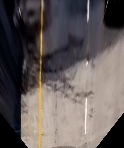 |
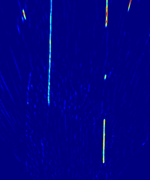
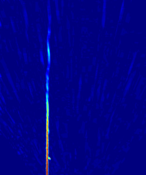
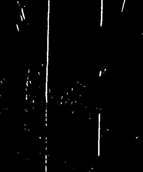
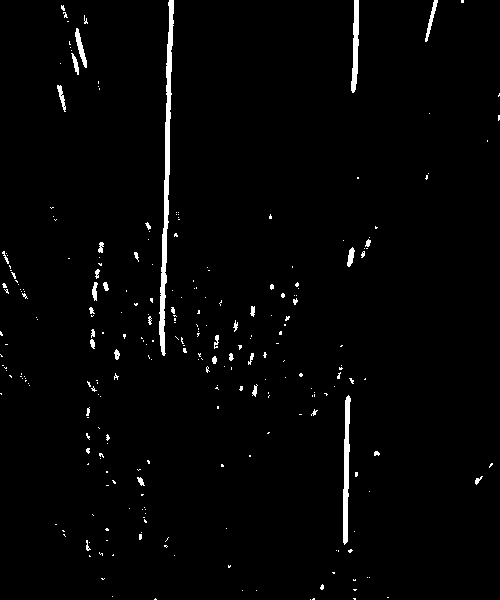
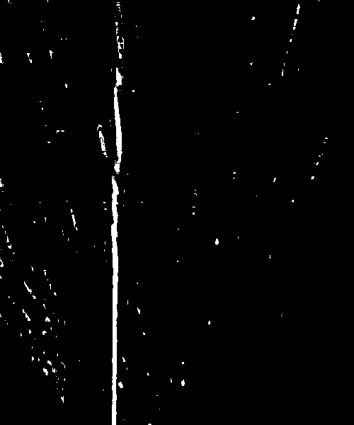
####2. Finding bright or yellow areas To find the bright or yellow areas, the morphological TOP HAT operation is used. It isolates the areas brighter than their surroundings. This operation is used in order to make pipeline robust against the lighting changes. In selected case, the lightness of the road surface changes, but we'll see that it does not affect the tophat morphological operation. The edge detection not used since they are extremely affected by the noise on the image, which makes them unsuitable for harder challenges. After applying TOP HAT operation, the image is thresholded using adaptive threshold which adds a bit more to the overall robustness. This part is implemented in lines 225 to 237. The resulting images are:
| Tophat on L channel from LAB | Tophat on L channel from HLS | Tophat on B channel from LAB |
|---|---|---|
 |
 |
 |
| Tophat on L channel from LAB | Tophat on L channel from HLS | Tophat on B channel from LAB |
 |
 |
 |
####3. Calculating single mask and passing it to the LaneLineFinder
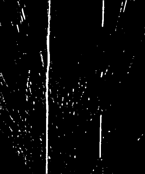
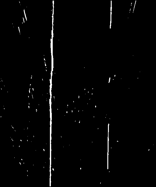
Once the masks are calculated, logical or is applied between them in order to obtain the total mask. Since the threshold is kept quite low, there will be a lot of noise. To avoid noise interfering with lane finding procedure, the mask is eroded which removes all the regions smaller than the structuring element. Once that is finished the masks are passed to LaneLineFinder which actually looks for the line in the binary image. This part is implemented from line 236 to line 248. The results are:
| Total mask | Eroded mask |
|---|---|
 |
 |
####4. Finding the line in a mask and fitting polynomial
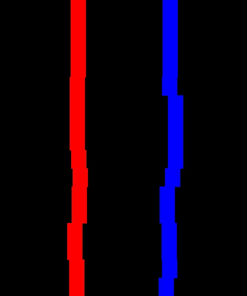
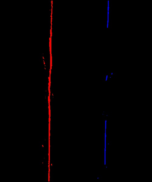
When the mask is found, the search for the line begins. The initial point to start a search is somewhere 1.82 meters (6 feet). Under the assumption that lane is 12feet wide and that the car is in its middle, we would be spot on. Since that might not hold, the search is performed in its surroundings. The window at the bottom of the image with the highest number of points included found. After that, we go one layer up and perform the same search but right now, we start from the maximum from the layer below. The search is performed until the top of the image is reached, gradually eliminating points outside of the maximal region. Function that does this is LaneLineFinder.find_lane_line(). After the lane points have been isolated, the polynomial fit is performed using LaneLineFinder.fit_lane_line(). In that procedures some statistics are calculated which help determine if the found line is good or not. The statistics include:
- Number of points in the fit
- Quality of the fit calculated using covariance matrix returned by
numpy.polyfit - Curvature of the road
- How far lane is from the center of the car
All of these have to be above some empirically defined threshold. The maximal regions and points used for fitting are shown in the image below (red is for left, blue is for right line):
| Line mask | Line points |
|---|---|
 |
 |
####5. Draw lane on original image and calculate curvature
If lanes are found, the curvature and position of the centre of the car is calculated using functions get_curvature() and get_center_shift(). Since the two lines are present, for the coefficient of the polynomial the mean value is used. The y coordinate for which the polynomials are evaluated is the bottom of the image. After that, the lines are drawn on a warped image and then unwarped and added to the original image. The last thing is to print out the values of curvature and offset of the center of the car. Results for all provided images can be found in output_images. Here is the result for discussed case:
| Warped lines | Final result |
|---|---|
 |
 |