Quantum optimal control made easy.
We go through life interacting with mechanisms that are controlled. For example, cruise control in a car will maintain a specific speed by appropriately applying fuel into the engine (or breaking). Of course, for the car to understand when it should apply fuel, it must have some feedback (closed-loop control)-- such as the speedometer. There are systems that do not need feedback (open-loop control), such as an electric clothes dryer that will continue operating for some time, regardless of clothes dryness.
Quantum systems, such as quantum computers, have parameters that we can control -- similar to the injection of fuel to a car engine, or the amount of heat to generate for an electric clothes dryer. The goal of quantum optimal control is to produce a desired operation (e.g. a quantum gate, or a quantum state) by computing pulses.
There are already many quantum optimal control software packages out in the universe. Pulses.jl attempts to be tiny (under 100 lines of code!), while also being quite powerful. We achieve this by utilizing Julia and the Julia ecosystem, such as:
] activate .
target = [...;...]
system = System(H_d, [H_c, ...])
initial_pulse = [...]
sol = Pulses.find_pulse(target, system, Δt, inital_pulse)
You may find more examples in examples.
Here are some examples and visualizations that were generated with Pulses.jl. The system Hamiltonians are taken to be superconducting Transmons.
Namely, the problem is the find pulses
The goal is to find
We want the Hadamard gate, which in matrix form is:
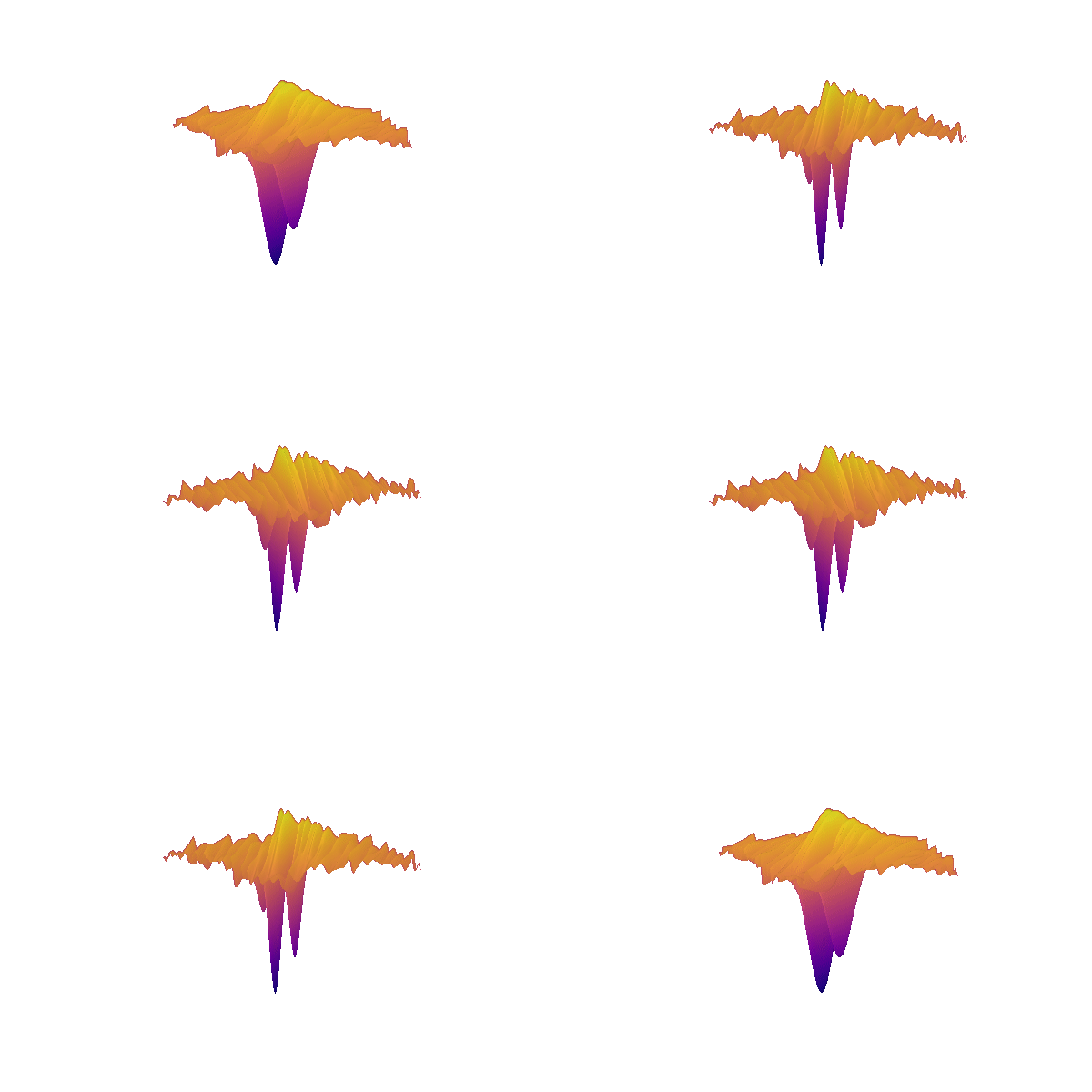
Pulses.jl finds the minimum of this loss landscape:
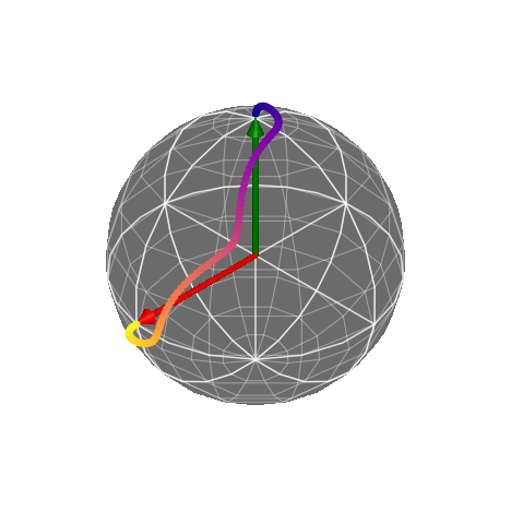
We then plot the found pulses, and also evolve a qubit in time using the pulses. Namely, starting in the state
Plot of
We want the CNOT gate, which in matrix form is:
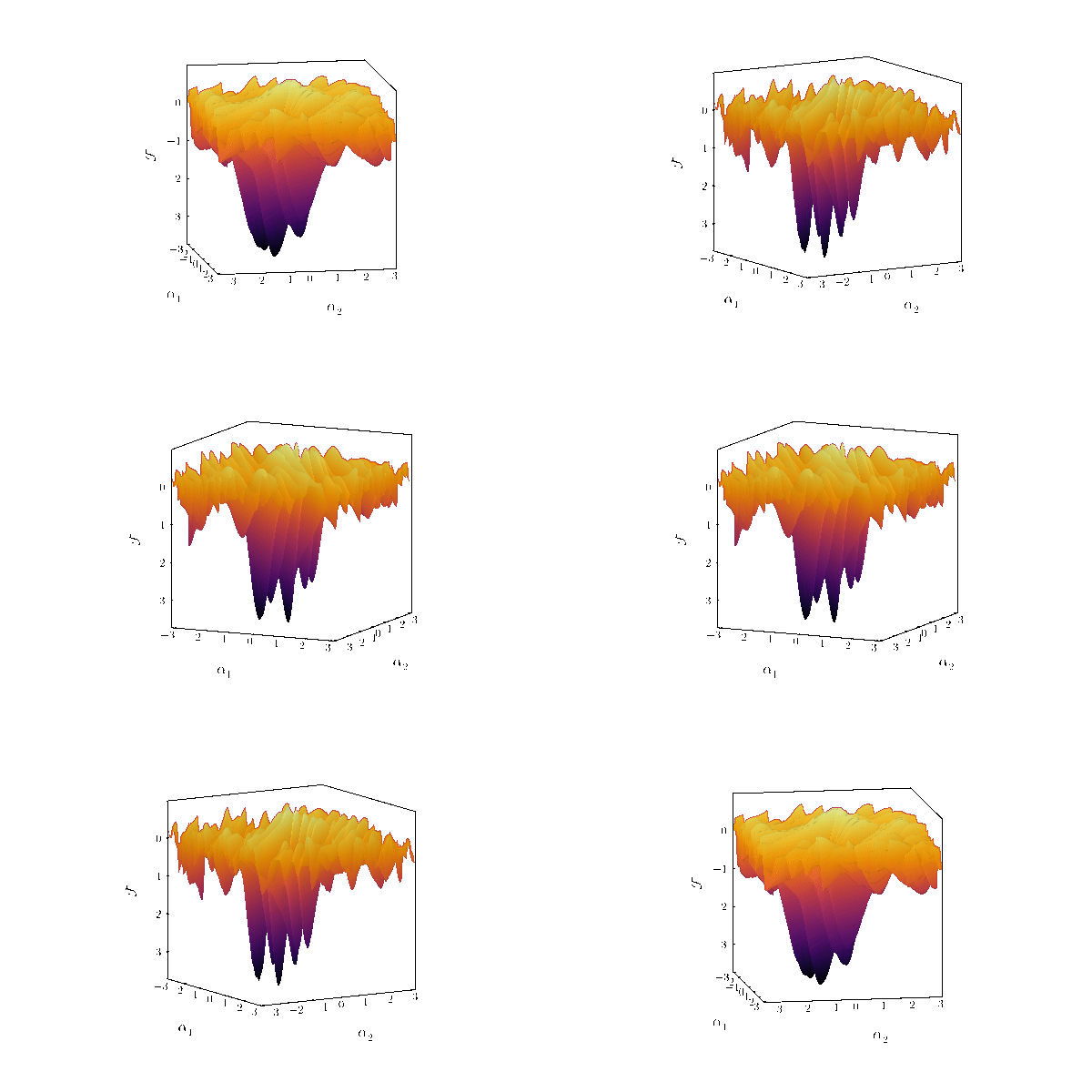
Pulses.jl finds the minimum of this loss landscape:
We then plot the evolution of the gate
@software{Volya_Pulses_jl_A_tiny_2022,
    author = {Volya, Daniel},
    title = {{Pulses.jl: A tiny quantum optimal control library.}},
    month = {12},
    year = {2022},
    publisher = {Zenodo},
    url = {https://github.com/RustyBamboo/Pulses.jl},
}
Distributed under the MIT License. See LICENSE for more information.


