In this project, a power bi based visualization app is proposed to analyze the spatial aspects of the dataset using Quality Spatial Relations (QSR). Two datasets have been used to be analysed under Monte Carlo Tree Search (MCTS) and also other popular Machine Learning algorithms. MCTS uses a UCB (Upper Confidence Bound) based reward system that simulates within the state space of every dataset.
From Speech project, The RAVDESS dataset based on the paper The Ryerson Audio-Visual Database of Emotional Speech and Song (RAVDESS) has been analysed using speech_sigproc.py.
From OCR project, The FUNSD Dataset based on the paper FUNSD Paper has been pre-processed using preprocess.py.
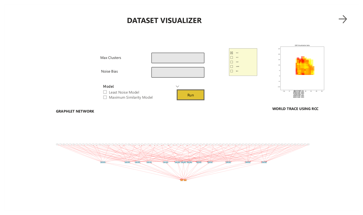
The App main page is a QSR visualizer page. When the maximum clusters are provided, the app asks for reward bias as well for input to MCTS simulation.
./speech/state_space/qsr.sh -d all
This command shows the final QSR plot after going through a 2 epoch training loop with Speech dataset, and another training loop with all distributions.
QSR Visualizer provides 2 plots:
- A Calculus plot (involving Region Connection Calculus (RCC), Ternary Point Configuration Calculus (TPCC))
- A Graphlet (involving temporal information integrated with the calculus)
All .npy files within tmp_models form the World Trace objects.
python ./speech/state_space/factor_analysis.py --n_iter=20000 --learning_rate=0.001 --filepath=./speech/state_space/models/factor_analysis.onnx
import onnxruntime as nxrun
sess = nxrun.InferenceSession("./speech/state_space/models/factor_analysis.onnx")

results = sess.run(None, {'latent': np.load('speech/dataset/latent.npy')})A state space model consisting of features and labels are fed into an MCTS algorithm. The state space model for each dataset consists of observations and transitions. When the data transitions to another state from an initial random state, the UCB model which is a multi-armed action bandit model, executes a Monte Carlo learning for n simulations. After obtaining the final state from an input state, the final state looks at the defined clusters which are ordered by a chosen metric. The number of maximum clusters are defined in the app's user interface. The maximum clusters should not exceed the state space dimension of the input data.
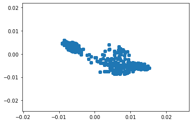
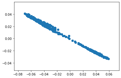
Observations are inferences from the feature extraction stage. Let's say we converted Audio signals into 120 mels, and then execute a FastICA on the mels, we get a dimensionality reduced mixing matrix plotted as a point cloud plot as shown:
Transitions are estimated factors assumed to be hierarchical which are derived from the observations. The factors obtained are Gaussian in nature and they are vectorized into speech/state_space/models/factor_analysis.onnx model.
The Monte Carlo Tree Search Algorithm updates the rewards based on the end result obtained instead of its online counterpart Temporal Difference Learning, TD (lambda). The algorithm clusters using ward linkage, with a maximum clusters parameter.
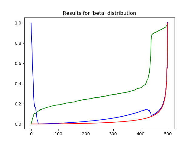
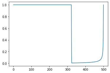
Here are the results shown during training of the Reward Scores, No. of Units, Chosen probability density function:
Below is the beta plot used for speech:
Below is the weibull distribution used for OCR:
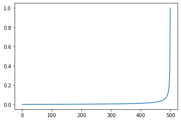
Below is the no. of units used for calibration of weibull:
For a dataset, the feature extraction is the first step. An Expectation Maximisation step has likelihoods in various forms. For factor analysis, there is a marginal likelihood; for dirichlet processes, the likelihood is a differential equation.
The episode scores obtained from running the MCTS algorithm, must be sorted in order to create a time series data for QSR analysis. The timestamps will be corresponding to argsort() of episode_scores. The rewards are hierarchical in nature, and hence the sorting of the scores are performed.
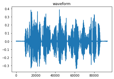
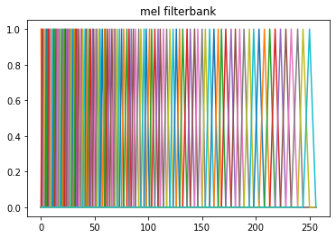
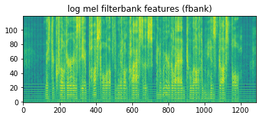
For evaluating the features from audio, the log mel spectrum and mel filterbank are produced. A hamming window is used to process the audio.
Audio Signal
Mel Filterbank
Mel Spectrum
In the data wrangling stage, the data is processed through a complex plane where there is timestamp information recorded from the output of UCB scores from a Monte Carlo Simulation. Also, the time series is unit spaced with each recorded variable being:
- no. of units required for calibration,
- the chosen probability density function,
- scores that are scaled from 0 to 1
A probability density function is chosen because it can maximise the likelihood of a statistical model for a given use case. In the case of factor analysis, when the data is decomposed into its latent space, there are two Gaussian models which express the ground truth in terms of how the overall model can capture the variance. If a statistical model is compared against a probability density function, the QSR visualizer can estimate time, a histogram of intervals and a histogram of QSR relations.
In a multi-armed bandit framework, a person simulates the environment by taking actions from a multi-labeled data source. The reward tree structure considers two approaches that have been documented based on:
- Least Noise model, in the case of Factor Analysis
- Maximum Similarity model, in the case of Latent Semantic Analysis
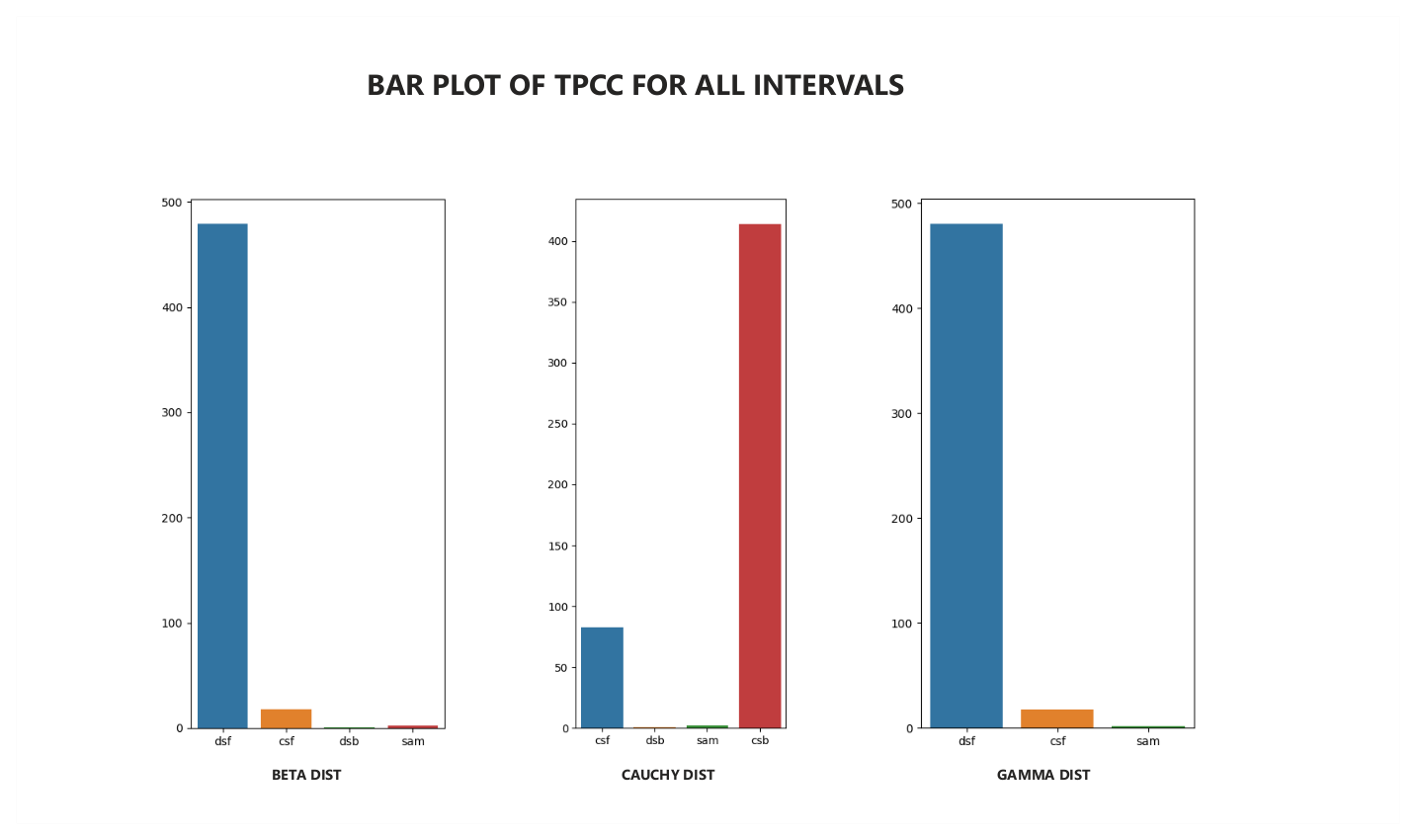
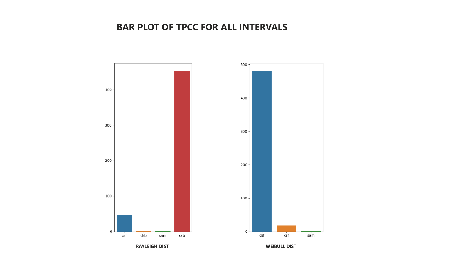
These results are obtained after executing a TPCC (Ternary Point Configuration Calculus) algorithm on the World Trace. Each Graphlet is an intermediary layer that computes the Allen relation among the world traces.
The net time taken to produce the Qualitative Spatio-Temporal Activity Graph (QSTAG)
Time: 0.100687980652
number of eps: 39
Histogram of Graphlets:
[20, 16, 13, 16, 16, 16, 2, 2, 2, 2, 1, 1, 1, 1, 2, 1, 1, 1]
The net time taken to produce the Qualitative Spatio-Temporal Activity Graph (QSTAG)
Time: 8.43655991554
number of eps: 146
Histogram of Graphlets:
[70, 69, 73, 1, 70, 66, 69, 1, 2, 2, 2, 2, 2, 2, 1, 1, 1, 1]
Time: 0.0908880233765
number of eps: 37
Histogram of Graphlets:
[19, 16, 14, 16, 16, 2, 16, 2, 2, 2, 2, 1]
Time: 1.20572209358
number of eps: 89
Histogram of Graphlets:
[45, 41, 41, 38, 41, 41, 2, 2, 2, 1, 1, 2, 1, 2, 1, 1, 1, 1]
Time: 0.0927407741547
number of eps: 37
Histogram of Graphlets:
[19, 16, 14, 16, 16, 2, 16, 2, 2, 2, 2, 1]
