Torch-Kalman

Time-series forecasting models using Kalman-filters in PyTorch.

Table of Contents

• Installation
• Example: Beijing Multi-Site Air-Quality Dataset
  • Prepare Our Dataset
  • Specify Our Model
  • Visualize the Results
  • Using Predictors

Installation

pip install git+https://github.com/strongio/torch-kalman.git#egg=torch_kalman

Example: Beijing Multi-Site Air-Quality Dataset

This dataset comes from the UCI Machine Learning Data Repository. It includes data on air pollutants and weather from 12 sites. To simplify the example, we'll focus on weekly averages for two measures: PM10 and SO2. Since these measures are strictly positive, we log-transform them.

df_aq_weekly.loc[:,['date','station','SO2','PM10','TEMP','PRES','DEWP']]

	date	station	SO2	PM10	TEMP	PRES	DEWP
0	2013-02-25	Aotizhongxin	36.541667	57.791667	2.525000	1022.777778	-15.666667
1	2013-03-04	Aotizhongxin	65.280906	198.149701	7.797619	1008.958929	-7.088690
2	2013-03-11	Aotizhongxin	57.416667	177.184524	6.402976	1014.233929	-2.277976
3	2013-03-18	Aotizhongxin	19.750000	92.511905	4.535119	1009.782738	-5.529762
4	2013-03-25	Aotizhongxin	41.559006	145.422619	6.991071	1012.829762	-3.762500
...	...	...	...	...	...	...	...
2515	2017-01-30	Wanshouxigong	27.666667	119.059524	0.768304	1024.101984	-18.331548
2516	2017-02-06	Wanshouxigong	15.544910	61.395210	0.625298	1025.392857	-16.977381
2517	2017-02-13	Wanshouxigong	26.166667	139.613095	2.870238	1019.840476	-11.551190
2518	2017-02-20	Wanshouxigong	7.020833	46.372414	3.425000	1022.414881	-11.811905
2519	2017-02-27	Wanshouxigong	9.613636	52.955556	9.647917	1016.014583	-9.964583

2520 rows × 7 columns

Prepare our Dataset

One of the key advantages of torch-kalman is the ability to train on a batch of time-serieses, instead of training a separate model for each individually. The TimeSeriesDataset is similar to PyTorch's native TensorDataset, with some useful metadata on the batch of time-serieses (the station names, the dates for each).

# preprocess our measures of interest:
measures = ['SO2','PM10']
measures_pp = [m + '_log10_scaled' for m in measures]
df_aq_weekly[measures_pp] = np.log10(df_aq_weekly[measures] / col_means[measures])

# create a dataset:
dataset_all = TimeSeriesDataset.from_dataframe(
    dataframe=df_aq_weekly,
    dt_unit='W',
    measure_colnames=measures_pp,
    group_colname='station', 
    time_colname='date',
    pad_X=0.0
)

# Train/Val split:
dataset_train, dataset_val = dataset_all.train_val_split(dt=SPLIT_DT)
dataset_train, dataset_val

(TimeSeriesDataset(sizes=[torch.Size([12, 156, 2])], measures=(('SO2_log10_scaled', 'PM10_log10_scaled'),)),
 TimeSeriesDataset(sizes=[torch.Size([12, 54, 2])], measures=(('SO2_log10_scaled', 'PM10_log10_scaled'),)))

Specify our Model

The KalmanFilter subclasses torch.nn.Module. We specify the model by passing processes that capture the behaviors of our measures.

processes = []
for measure in measures_pp:
    processes.extend([
        LocalTrend(
            id=f'{measure}_trend', multi=.01
        ).add_measure(measure),
        LocalLevel(
            id=f'{measure}_local_level',
            decay=(.90,1.00)
        ).add_measure(measure),
        FourierSeason(
            id=f'{measure}_day_in_year', seasonal_period=365.25 / 7., dt_unit='W', K=2, fixed=True
        ).add_measure(measure)
    ])
kf_first = KalmanFilter(measures=measures_pp, 
                      processes=processes, 
                      measure_var_predict=('seasonal',dict(K=2,period='yearly',dt_unit='W')))

Here we're showing off a few useful features of torch-kalman:

• We are training on a multivarite time-series: that is, our time-series has two measures (SO2 and PM10) and our model will capture correlations across these.
• We are going to train on, and predictor for, multiple time-serieses (i.e. multiple stations) at once.
• We are allowing the amount of noise in the measure (i.e., the measure variance) to vary with the seasons, by passing 'seasonal' alias to measure_var_predict. (The measure_var_predict argument takes any torch.nn.Module that can be used for prediction, but 'seasonal' is an alias that tells the KalmanFilter to use a seasonal NN.)

Train our Model

When we call our KalmanFilter, we get predictions (a StateBeliefOverTime) which come with a mean and covariance, and so can be evaluated against the actual data using a (negative) log-probability critierion.

kf_first.opt = LBFGS(kf_first.parameters(), lr=.20, max_eval=10)

def closure():
    kf_first.opt.zero_grad()
    pred = kf_first(
        dataset_train.tensors[0], 
        start_datetimes=dataset_train.start_datetimes, 
    )
    loss = -pred.log_prob(dataset_train.tensors[0]).mean()
    loss.backward()
    return loss

for epoch in range(15):
    train_loss = kf_first.opt.step(closure).item()
    with torch.no_grad():
        pred = kf_first(
            dataset_val.tensors[0], 
            start_datetimes=dataset_val.start_datetimes
        )
        val_loss = -pred.log_prob(dataset_val.tensors[0]).mean().item()
    print(f"EPOCH {epoch}, TRAIN LOSS {train_loss}, VAL LOSS {val_loss}")

EPOCH 0, TRAIN LOSS 2.372123956680298, VAL LOSS 1.0876796245574951
EPOCH 1, TRAIN LOSS 0.4992632269859314, VAL LOSS -0.6029616594314575
EPOCH 2, TRAIN LOSS -0.6929754018783569, VAL LOSS -0.6424744725227356
EPOCH 3, TRAIN LOSS -0.7372146248817444, VAL LOSS -0.6508392691612244
EPOCH 4, TRAIN LOSS -0.7536402940750122, VAL LOSS -0.6748760342597961
EPOCH 5, TRAIN LOSS -0.7693123817443848, VAL LOSS -0.7698904871940613
EPOCH 6, TRAIN LOSS -0.8141641020774841, VAL LOSS -0.7885841131210327
EPOCH 7, TRAIN LOSS -0.8502019643783569, VAL LOSS -0.7430527210235596
EPOCH 8, TRAIN LOSS -0.8761543035507202, VAL LOSS -0.6768094301223755
EPOCH 9, TRAIN LOSS -0.8880344033241272, VAL LOSS -0.6236486434936523
EPOCH 10, TRAIN LOSS -0.9021796584129333, VAL LOSS -0.6441830992698669
EPOCH 11, TRAIN LOSS -0.9108285307884216, VAL LOSS -0.6910713315010071
EPOCH 12, TRAIN LOSS -0.9218556880950928, VAL LOSS -0.6219266057014465
EPOCH 13, TRAIN LOSS -0.9351726174354553, VAL LOSS -0.6124213337898254
EPOCH 14, TRAIN LOSS -0.9403404593467712, VAL LOSS -0.6187482476234436

Visualize the Results

def inverse_transform(df: pd.DataFrame, col_means: pd.Series) -> pd.DataFrame:
    df = df.copy()
    df['measure'] = df['measure'].str.replace('_log10_scaled','')
    std = (df['upper'] - df['lower']) / 1.96
    for col in ['mean','lower','upper','actual']:
        if col == 'mean':
            # bias correction:
            df[col] = df[col] + .5 * std ** 2
        df[col] = 10 ** df[col] # inverse log10
        df[col] *= df['measure'].map(col_means.to_dict()) # inverse scaling
    return df

pred = kf_first(
    dataset_train.tensors[0], 
    start_datetimes=dataset_train.start_datetimes,
    out_timesteps=dataset_all.tensors[0].shape[1]
)

df_pred = inverse_transform(pred.to_dataframe(dataset_all), col_means)

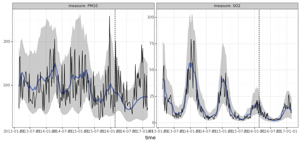
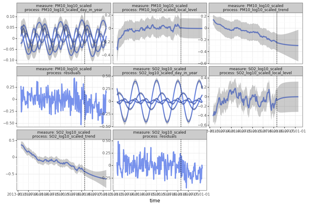
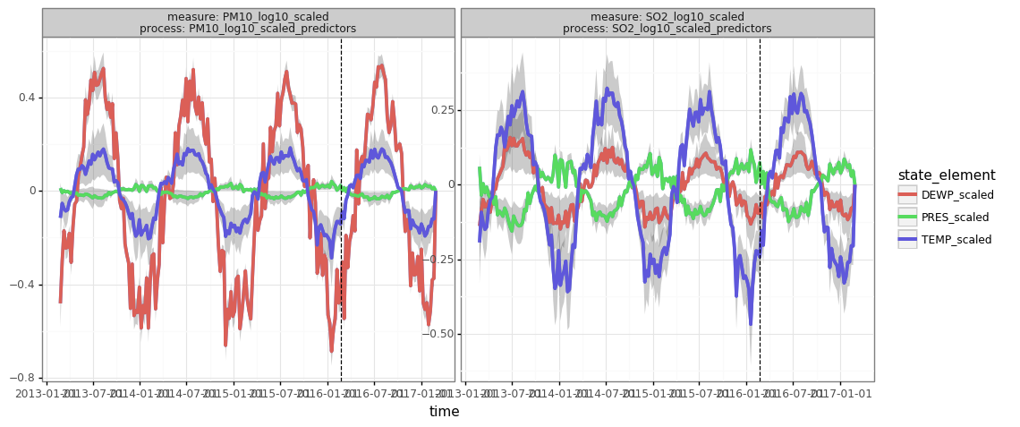
print(pred.plot(df_pred.query("group=='Changping'"), split_dt=SPLIT_DT))

print(pred.plot(pred.to_dataframe(dataset_all, type='components').query("group=='Changping'"), split_dt=SPLIT_DT))

Using Predictors

Here, we'll use the weather to predict our measures of interest. We add these predictors by adding a LinearModel process to our model. torch-kalman also supports using any neural network to generate latent states for our model -- see the NN process.

predictors = ['TEMP', 'PRES', 'DEWP']
predictors_pp = [x + '_scaled' for x in predictors]

df_aq_weekly[predictors_pp] = (df_aq_weekly[predictors] - col_means[predictors]) / col_stds[predictors]

dataset_all = TimeSeriesDataset.from_dataframe(
    dataframe=df_aq_weekly,
    dt_unit='W',
    group_colname='station',
    time_colname='date',
    y_colnames=measures_pp,
    X_colnames=predictors_pp
)

dataset_train, dataset_val = dataset_all.train_val_split(dt=SPLIT_DT)

# impute nans (since standardized, imputing w/zeros means imputing w/mean)
for _dataset in (dataset_all, dataset_train, dataset_val):
    _, X = _dataset.tensors
    X[torch.isnan(X)] = 0.0

kf_pred = KalmanFilter(
    measures=measures_pp,
    processes=processes + [
        LinearModel(id=f'{m}_predictors', covariates=predictors_pp).add_measure(m) 
        for m in measures_pp
    ]
)

kf_pred.opt = LBFGS(kf_pred.parameters(), lr=.20, max_eval=10)

def closure():
    kf_pred.opt.zero_grad()
    y, X = dataset_train.tensors
    pred = kf_pred(y, predictors=X, start_datetimes=dataset_train.start_datetimes)
    loss = -pred.log_prob(y).mean()
    loss.backward()
    return loss

for epoch in range(20):
    train_loss = kf_pred.opt.step(closure).item()
    y, X = dataset_val.tensors
    with torch.no_grad():
        pred = kf_pred(y, predictors=X, start_datetimes=dataset_val.start_datetimes)
        val_loss = -pred.log_prob(y).mean().item()
    print(f"EPOCH {epoch}, TRAIN LOSS {train_loss}, VAL LOSS {val_loss}")

y, _ = dataset_train.tensors # only input air-pollutant data from 'train' period
_, X = dataset_all.tensors # but provide exogenous predictors from both 'train' and 'validation' periods
pred = kf_pred(
    y, 
    predictors=X, 
    start_datetimes=dataset_train.start_datetimes,
    out_timesteps=X.shape[1]
)

print(
    pred.plot(inverse_transform(pred.to_dataframe(dataset_all).query("group=='Changping'"), col_means),split_dt=SPLIT_DT)
)

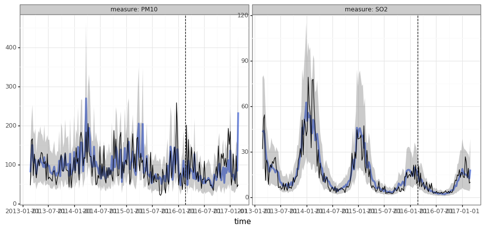
df_components = pred.to_dataframe(dataset_all, type='components')

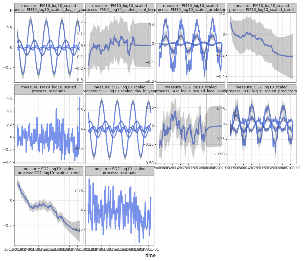
print(pred.plot(df_components.query("group=='Changping'"), split_dt=SPLIT_DT))

print(pred.plot(df_components.query("(group=='Changping') & (process.str.endswith('predictors'))"), split_dt=SPLIT_DT))