Summary:
Canapy dashboard and tools can be installed using pip (python installation package). You can install canapy using one of these two options:
If you do not have pip you can found info here to install it.
1st option to install canapy (local copy)
git clone [email protected]:birds-canopy/canapy.git
pip install -e canapy/.
or replace the second command line by this one if you want to install from another path (where you cloned the canapy repository):
pip install -e <path to canapy directory containing pyproject.toml>2nd option to install canapy
pip install -e git+https://github.com/birds-canopy/canapy.git#egg=canapy-rebornCanapy uses supervised machine learning tools to create automatic annotators, and thus requires some hand-made annotations to bootstrap the annotation pipeline. Using our proposed method, we recommend to ideally have between 30 minutes and 1 hour of annotated sounds to train an automatic annotator - but from our experiments on canary data with 10 min of songs you can already obtain nice results! This may of course vary depending on the nature of the annotated vocalizations. Canapy was primarily designed to annotate bird songs, in particular domestic canary songs.
Two sources of data are required to train an annotator: annotations and audio.
Annotations are typically segments of audio labeled using a custom code representing different vocal units, like phonemes, syllables or words in human speech. In their most essential form, they are defined using the triplet (onset, offset, label), representing an annotated segment, delineated in time.
For the time being, canapy only deals with non-overlapping annotation segments, and can thus only work on a single track of annotations.
This format is inspired by the M1-spring dataset, a dataset of more than 400 hand-labeled songs of one domestic canary. It's a simple, straightforward format, that is best expressed in a comma-separated values spreadsheet (.csv file).
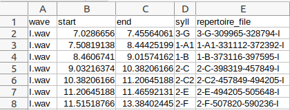
Four named columns of data are needed to define an annotation:
wave: the name of the audio track being annotated.start: the beginning of the annotation on the audio track, in secondsend: the end of the annotation on the audio track, in secondssyll: the annotation label
Warning
TODO change screenshot
An example .csv file may look like this:
Audio annotations come in many different formats these days. You may have used Audacity, Raven, or Praat to annotate your data by hand.
By default, canapy uses its own annotation format, called marron1csv, to process annotation data. To allow using a different format, canapy was built on top of crowsetta, an audio annotation formats managing tool, which can handle many different annotation format coming from many different annotation software. We recommend diving into crowsetta documentation to learn more about annotation formats.
Audio recordings handled by canapy can have any sampling frequency. They must be mono audio recordings. If stereo audio are provided, they will be converted to mono.
Canapy currently works with two audio data formats: WAV files (.wav) and Numpy arrays (.npy).
When creating new automatic annotators for your data, you should provide some hand-labeled audios in order to train canapy to annotate this data.
Because canapy will try to split your dataset in two parts (one for training and one to test its capabilities), you should provide several audio and annotation files. Canapy will consider each audio file as one sequence of vocalizations, and will never cut this sequence when training or annotating. When dealing with songbirds for instance, one file should ideally contain a single song sequence.
Your dataset should therefore looks something like this:
├── song_dataset
    └── annotations
        ├── song1.csv
        ├── song2.csv
        ...
        └── songN.csv
    ├── audio
        ├── song1.wav
        ├── song2.wav
        ...
        └── songN.wav
Here, .csv files in the annotations/ folder contain annotations in marron1csv format (depending on your annotation format you may have different file extension) and .wav files in the audio/ folder are your audio recordings in WAV format.
You can also provide audio recording and annotation files all mixed in a single directory:
├── song_dataset
    └── data
        ├── song1.csv
        ├── song1.wav
        ├── song2.csv
        ├── song2.wav
        ...
        ├── songN.csv
        └── songN.wav
Pay attention to how your audio files are named. Audio filenames
will be used by annotation tools to link annotations with their
corresponding audio. For instance, using the marron1csv annotation
format, all values in the wave column in the .csv files must match one of the
audio filenames.
Once training has been performed, your dataset may consist only of audio files. As no dataset split is required for annotating files, your dataset may be one single file, or several smaller files. We do not recommend using too long files however. Depending on your computer, using very long recordings may be suboptimal, or even crash the annotator.
The easiest way to train annotators and check the quality of the dataset if by canapy dashboard application.
To run the dashboard and load your dataset at song_dataset/, simply do:
canapy dash -a song_dataset/annotations -s song_dataset/audio -o outputor, if audio and annotations are placed in the same directory:
canapy dash -d song_dataset/data -o outputThe dashboard should open in your browser, at localhost:9321. If not, simply reach localhost:9321 in your favorite browser.
All the data produced by the dashboard (models and checkpoints) will be stored in output/.
The first dashboard you will see in the one devoted to train the model.
Click on the button Start training to begin the training of the annotators and then produce the annotations. Metrics should display in the terminal where you started the dashboard.
At the end of the training sequence, click on "Next step" to display the "eval" dashboard (it can take some time to display, don't worry, click only once on the button).
The first dashboard will train annotation models on the current version of the dataset, and produce their respective versions of the annotations.
Two models are built during the training phase. They both are based on an Echo State Network (ESN), a kind of artificial neural network, and have the same parameters. They are, however, trained on two different tasks:
- the syn model (syntactic model) is trained to annotate whole songs. Entire songs and annotations files are presented to the models during training. Thus, the model is trained only on the available data, meaning that imbalance in number between the categories of bird phrases is preserved. The model is also expected to rely on syntactic information to produce its annotations, being trained on the real order of the phrases in the songs.
- the nsyn model (non syntactic model) is trained to annotate only randomly mixed phrases, with an artificially balanced number of phrases samples. This model is expected to rely only on inner characteristics of each type of syllables to annotate the songs, without taking into account their context in the song. Imbalance in number is also not preserved, meaning the model has to give the same importance to all categories of syllables.
Finally, a third model, called ensemble, combine the outputs of the two previous models with a vote system, to combine the "judgements" of the two models in a new one.
The second dashboard displays the performances of the three models during the real annotation task: all three models are fed with the whole songs contained in the hand-annotated dataset, and we will now look at the differences between their annotations and the handmade ones.
This dashboard is divided in two parts:
- the Class merge dashboard
- the Sample correction dashboard You can switch between them with the buttons at the top of the dashboard.
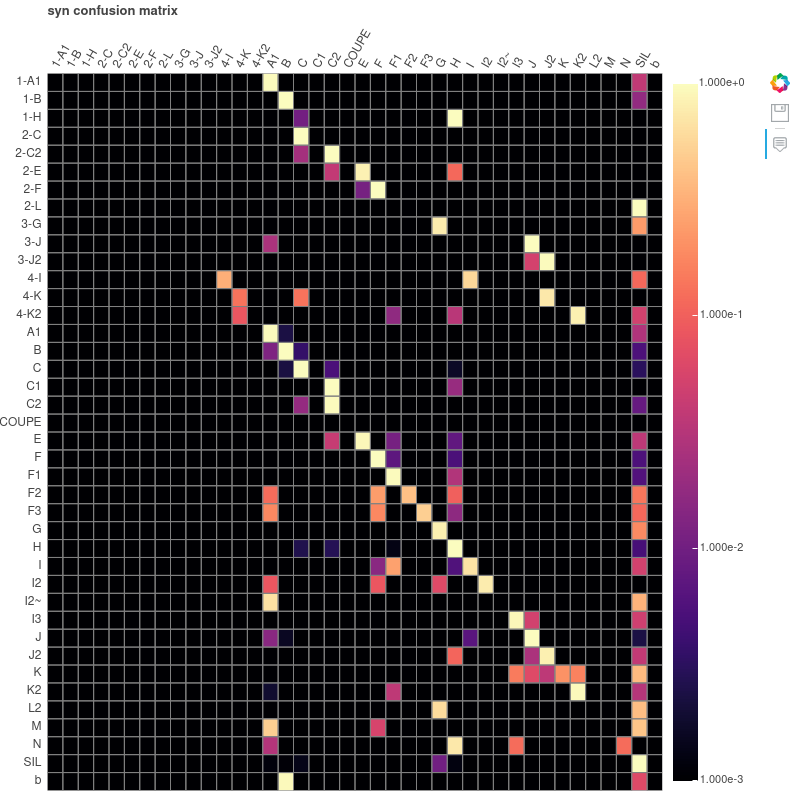
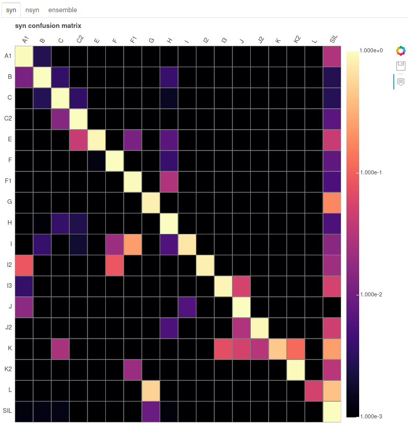
In the Class merge dashboard, you can use the confusion matrices to inspect syllables categories where the models make a lot of mistakes. If the mistake pattern seems stable (high confusion between two classes, and potential agreement between the models), this could be the sign that the confused categories could be merged into one. This happens a lot on handmade annotations, due to obvious spelling mistakes in the annotations labels, or to disagreement in the naming between the human annotators, or to "over-classification" of certain patterns.
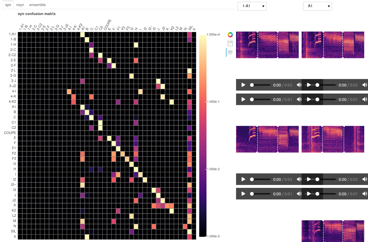 You can use the inspector at the right of the confusion matrices (clicking on the two buttons at the top right of the above screenshot) to display some class samples and see if a merge is coherent. When you have taken your decision, simply write the new name of the class you want to modify in the correction panel at the extreme right of the dashboard (for example, if you want to merge categories A and A1, because they are really close, simply write "A" under "A1" class text input).
If the class contains few samples and doesn't seem well-founded you can delete it by writing 'DELETE' in the text input under the name of the syllable category. Sometimes, some classes contains very few instances that are not sufficient for the model to recognize them, meaning they will not be usable. In this case making a 'TRASH' class is a good idea.
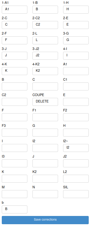
Make sure to click on the Save corrections button under the syllable types input text to save your changes.
Moreover, you can find help to make corrections while looking to the metrics indicated under the confusion matrix.
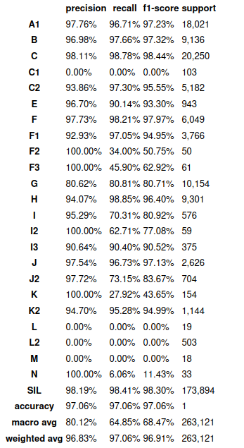
For example here the models achieve 97.06% accuracy each which is pretty good. However, you can see classes like C1, L, L2... that scores 0% in precision, recall and f1-score, meaning they may be deleted. If you choose to keep this model it will do a great job detecting the other classes but may lack experience recognizing the phrases labeled as C1, L,L2...
You can also inspect the samples about which the models disagree the most in the Sample correction dashboard. Here, all the annotations that are confused with another class over at least 2/3 of their time length by the models can be displayed, and manually corrected (the 2/3 time length disagreement parameter can be changed in the configuration file (see section 6.)).
Again, at the right of the bar plot showing the disagreements' distribution, an inspector allows you to display samples of all the categories of syllables.
The models aren't always right, as they use prediction you have the last word on which label to attribute to a phrase.
If the sample correction is empty, don't panic! it only means that the models performs well (maybe too well?) on the dataset. It is often the case with little datasets, where the models overfit the misrepresented categories of syllables. In any way, you should first focus on merging whole categories of syllables before correcting single samples.
Make sure to click on the Save all button on the right of the distribution figure to save your changes.
You have two choices then:
- click the
Next stepbutton. This will redirect you to the 'train' dashboard. Indeed, after you have applied corrections on the dataset, you should retrain the models to see the increase in performance, and to check if by changing the data distribution new disagreements do not appear. You should do 3-4 iterations of training-evaluating to be sure that you have fixed all the annotations. Below, the comparison of the initial confusion matrix of the syntactic model and its matrix after some corrections:
- click the
Exportbutton. If you are happy with the models performances and the annotations' distribution of the dataset, after some iterations, you can click on this button to be redirected to the 'export' dashboard. This dashboard will simply retrain all the models with all the corrections applied on the dataset, and save them in the output directory, with the correction file, the configuration file, etc.
In any case, a checkpoint of the current state of your analysis will be saved : corrections, configuration, models and annotations will be stored in the output/checkpoint directory, in a subdirectory named after the iteration number (1 if it is your first run, 2 if it is the second time you apply corrections and train models, and so on).
After training your model you will find in the output/ directory:
checkpoints: corrections, configuration, models and annotations corresponding to a round of training, in a subdirectory named after the iteration number (1if it is your first run,2if it is the second time you apply corrections and train models, and so on).models: 'syn' and 'nsyn' program corresponding to the final version of the syntactic and non syntactic models you have trained
Canapy is primarily a Python tool to build simple and fast automatic audio annotation pipelines, using a simple yet efficient machine learning technique: Reservoir Computing.
An annotation pipeline can be defined using two objects: the Corpus and the
Annotator.
The Corpus object is a representation of your dataset within canapy.
It holds reference to audio data, is in charge with loading and
formatting your annotations (when needed), and may also store some
other things like preprocessed data - spectrograms, for instance.
To load your dataset into a Corpus object, simply use:
from canapy import Corpus

corpus = Corpus.from_directory(
  audio_directory="song_dataset/audio/",
  annots_directory="song_dataset/annotations/"
)By default, the annotation format is marron1csv, but you may change
to any other format provided by crowsetta, using the annot_format
argument. You may also change the expected audio format using the audio_ext
argument, and setting it to ".wav" or ".npy" (respectively to
provide WAV files or Numpy arrays archive files).
corpus = Corpus.from_directory(
  audio_directory="song_dataset/audio/",
  annots_directory="song_dataset/annotations/",
  annot_format="aud-seq", # Audacity label track format
  audio_ext=".wav",  # Search for .wav files in the audio directory
)As explained in Prepare your data, you can also provide
a link to a single directory containing both annotations and audio, or create
an audio-only Corpus by omitting the annots_directory argument:
# Annotated corpus, all data in the
# same directory
corpus = Corpus.from_directory(
  audio_directory="song_dataset/data/",
  annots_directory="song_dataset/data/" # Same directory !
)

# Non-annotated corpus (only audio)
non_annotated_corpus = Corpus.from_directory(
  audio_directory="song_dataset/audio/",
)
The Corpus object will automatically format your data into crowsetta standard
annotation format generic-seq. This makes data formats interchangeable to some
extent. You can access a tabular representation of annotations (as a pandas.DataFrame)
from the dataset attribute:
print(corpus.dataset)Output:
    notated_path   onset_s    offset_s    label    annotation   sequence
0      song1.wav      1.20        1.42        A             0          0
1      song1.wav      1.55        2.12        B             0          0
2      song1.wav      2.41        2.79        C             0          0
3      song1.wav      2.89        3.45        A             0          0
The notated_path column keep tracks of the attached audio file.
The onset_s, offset_s, and label columns respectively store
annotation segments start, end, and label. All onsets and offsets
are expressed in seconds since the beginning of audio track.
The annotation and sequence columns are special
attributes of crowsetta generic-seq format, which we do not
directly use in canapy.
If your corpus is not annotated (only audio), the code above
will return None:
print(corpus.dataset)Output:
None
Corpus can be saved to disk as CSV files, one per audio file,
if they have annotations:
corpus.to_directory("/save_directory")Annotation in canapy is performed by an Annotator. There are several Annotator currently available, but the simplest one and the most useful is the SynAnnotator:
from canapy.annotator import SynAnnotator

annotator = SynAnnotator()
This object is in charge with training a
machine learning model able to annotate
your data, based on some audio and annotations
stored in a Corpus, and eventually annotate
a Corpus with unlabelled audio recordings.
After creating an annotated Corpus object,
you may .fit your annotator to your
dataset:
annotator.fit(corpus)This trains the annotator on your dataset.
You may access the labels learned by the
annotator from the .vocab attribute:
print(annotator.vocab)You can save an annotator on your computer using
the .to_disk method:
annotator.to_disk("save_directory/annotator")After having saved an annotator on your computer, you
can load it again using the .from_disk method of the
Annotator base class:
from canapy.annotator import Annotator

annotator = Annotator.from_disk("saved_directory/annotator") You may now annotate unlabeled audio the .predict method
of your annotator, generating a new Corpus with freshly
computed annotations:
# Load some unlabelled data
corpus = Corpus.from_directory(audio_directory="song_data/audio")

# Annotate !
labeled_corpus = annotator.predict(corpus)

print(labeled_corpus.dataset)

# Additionally save your annotated `Corpus`
labeled_corpus.to_directory("song_data/new_annotations")Canapy configuration is stored in configuration files in TOML format. They are human readable, and it is possible to comment them for additional clarity.
You can access canapy default configuration from config.default_config:
from config import default_config

print(default_config)

# It's basically a big nested dictionary of values
print(default_config.transforms.annots.time_precision)The best way to quickly change some parameters, such as the audio sampling rate, is to change them directly from the default configuration.
First, import the default configuration, and then change the parameter you wish to change:
from copy import deepcopy
from config import default_config

# Copy the default configuration
my_config = deepcopy(default_config)

# Change the audio sampling frequency
# to 16000Hz
my_config.transforms.audio.sampling_rate = 16000
The objects in charge with dealing with the configuration throughout
your annotation pipeline are your Corpus and Annotator. To apply your
configuration, change your Corpus configuration files:
corpus = Corpus.from_directory(audio_directory="song_dateset/audio")
# Apply your configuration
corpus.config = my_config
And give your configuration as parameter to your Annotator:
annotator = SynAnnotator(config=my_config)As configuration files are necessary to your pipelines,
we recommend to save your configuration as a TOML file
if you make any change to the default configuration,
using the .to_disk method:
my_config.to_disk("saved_directory/my_config.toml")To create your own configuration file, start from the existing
default configuration, make some changes, and save it somewhere,
let's say at saved_directory/my_config.toml.
Warning
Do not change default parameter names! Most of them are required by canapy to work.
You can now load your configuration file directly from your Corpus
object, using the config_path argument:
corpus = Corpus.from_directory(
  annots_directory="song_dataset/annots",
  audio_directory="song_dataset/audio",
  config_path="saved_directory/my_config.toml")
You may now check that your Corpus .config is
identical to your personal configuration file:
print(corpus.config)You can finally inject this configuration file in your new Annotators:
annotator = SynAnnotator(config=corpus.config)You may also change the dashboard configuration
by providing this file as argument using the --config_path
parameter.
A configuration file looks like this. All the keys are mandatory:
[misc]
seed=42

[transforms.annots]
time_precision=0.001 # seconds
min_label_duration=0.02 # seconds
lonely_labels=["cri", "TRASH"]
min_silence_gap=0.001 # seconds
silence_tag="SIL"

[transforms.audio]
audio_features=["mfcc", "delta", "delta2"]
sampling_rate=44100 # Hz
n_mfcc=13
hop_length=0.01 # seconds
win_length=0.02 # seconds
n_fft=2048 # audio frames
fmin=500 # Hz
fmax=8000 # Hz
lifter=40

[transforms.audio.delta]
padding="wrap"

[transforms.audio.delta2]
padding="wrap"

[transforms.training]
max_sequences=-1
test_ratio=0.2

[transforms.training.balance]
min_class_total_duration=2  #30 # seconds
min_silence_duration=0.2 # seconds

[transforms.training.balance.data_augmentation]
noise_std=0.01

[model.syn]
units=1000
sr=0.4
leak=0.1
iss=0.0005
isd=0.02
isd2=0.002
ridge=1e-8
backend="multiprocessing"
workers=-1

[model.nsyn]
units=1000
sr=0.4
leak=0.1
iss=0.0005
isd=0.02
isd2=0.002
ridge=1e-8
backend="multiprocessing"
workers=-1

[correction]
min_segment_proportion_agreement=0.66- seed = 42: Defines the seed for random number generators to ensure reproducible results.
- time_precision = 0.001: Time accuracy of annotations, in seconds.
- min_label_duration = 0.02: Minimum duration of a label, in seconds. Labels shorter than this value will be ignored or merged.
- lonely_labels = [‘cri’, ‘TRASH’]: List of labels considered ‘isolated’ and which may require special treatment.
- min_silence_gap = 0.001: Minimum silence interval, in seconds, to separate two audio segments.
- silence_tag = ‘SIL’: Tag used to mark silence segments.
- audio_features = [‘mfcc’, ‘delta’, ‘delta2’]: List of audio features to be extracted, in this case the mel-frequency cepstral coefficients (MFCC) and their first and second derivatives.
- sampling_rate = 44100: Audio sampling rate, in Hertz.
- n_mfcc = 13: Number of MFCC coefficients to extract.
- hop_length = 0.01: Jump interval between analysis windows, in seconds.
- win_length = 0.02: Length of analysis window, in seconds.
- n_fft = 2048: Number of points for the Fast Fourier Transform (FFT), used to calculate the spectrogram.
- fmin = 500: Minimum frequency to be considered when extracting characteristics, in Hertz.
- fmax = 8000: Maximum frequency to be considered when extracting characteristics, in Hertz.
- lifter = 40: Parameter for lifting cepstral coefficients, often used to accentuate the high-frequency characteristics of MFCCs.
- padding = ‘wrap’: Padding method for first derivatives (delta), here using circular padding.
- padding = ‘wrap’: Padding method for second derivatives (delta2), here using circular padding.
- max_sequences = -1: Maximum number of sequences for training. -1 can mean that there is no limit.
- test_ratio = 0.2: Proportion of data used for the test, in this case 20%.
- min_class_total_duration = 2: Minimum total duration for each class when balancing data, in seconds.
- min_silence_duration = 0.2: Minimum duration of silence segments to consider when balancing data, in seconds.
- noise_std = 0.01: Standard deviation of noise added for data augmentation, here to simulate white Gaussian noise.
- units = 1000: Number of units in the recursive syn model.
- sr = 0.4: Spectral radius of recurrent weight matrix.
- leak = 0.1: Leakage parameter for recurrent units.
- iss = 0.0005: Parameter for MFCC input scaling.
- isd = 0.02: Parameter for MFCC derivatives input scaling.
- isd2 = 0.002: Parameter for MFCC second derivatives input scaling.
- ridge = 1e-8: Ridge regularisation parameter.
- backend = ‘multiprocessing’: Backend used for parallel calculation.
- workers = -1: Number of workers for the multiprocessing backend. -1 means using all available CPUs.
The same parameters as for [model.syn], applied to another recurrent model (nsyn).
- min_segment_proportion_agreement=0.66: Minimum proportion of agreement to consider a segment as valid when correcting annotations.
If you have any problems with using Canapy, don't hesitate to contact Nathan Trouvain or Albane Arthuis at Inria Mnemosyne team: [email protected] [email protected]