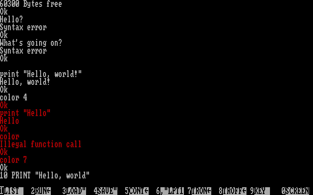
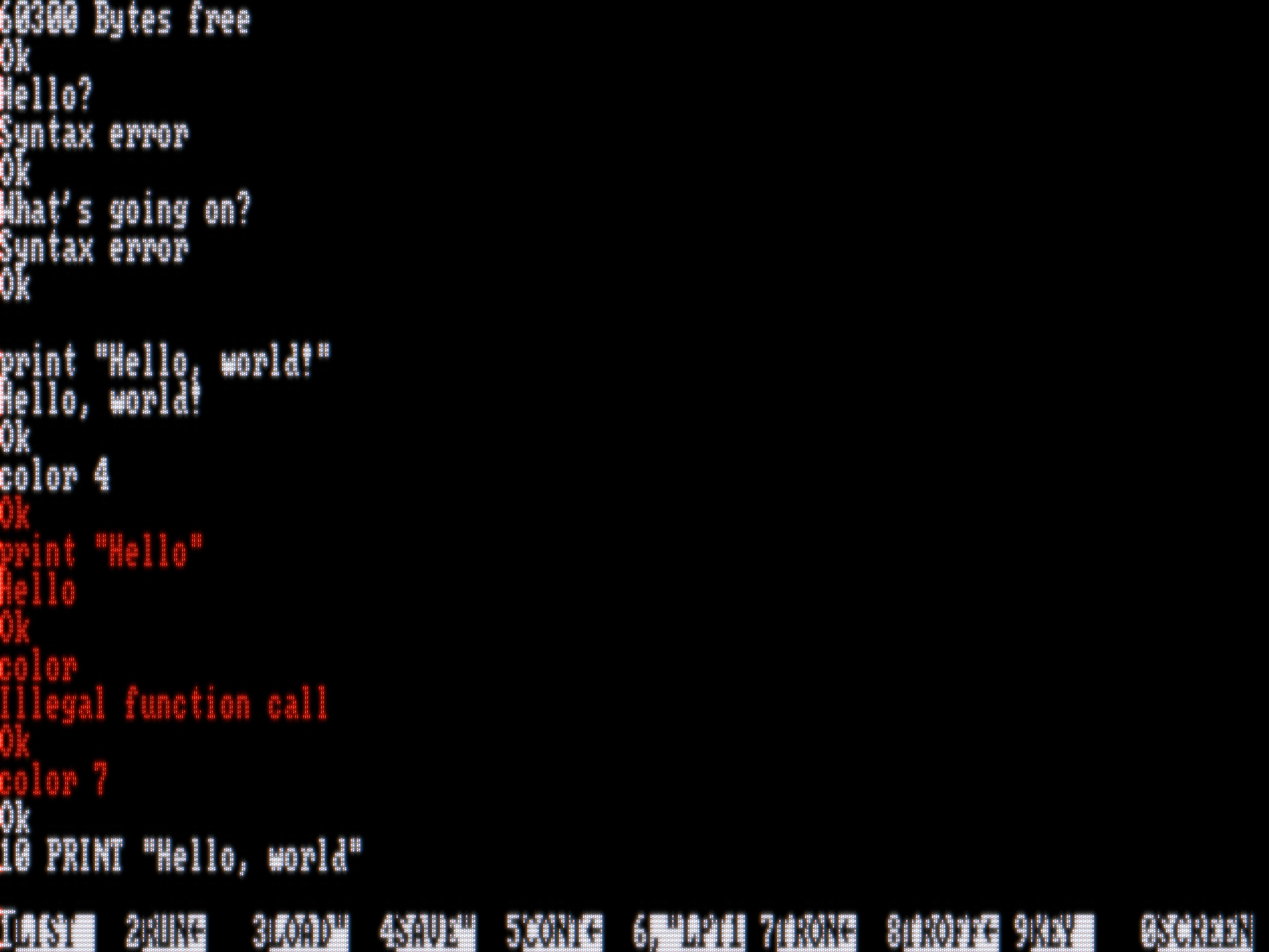
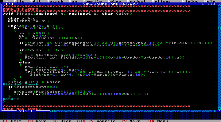
This is the CRT filter that I used in my ”What is That Editor” video, at https://www.youtube.com/watch?v=ZMBQmhO8KqI.
It received some accolades, but I forgot to publish it. Here it is finally.
Run this command to build the filter:
g++ -o crt-filter crt-filter.cc -fopenmp -Ofast -march=native -Wall -Wextra -std=c++17
The filter takes BGRA (RGB32) video (RAW!) from stdin, and produces BGRA video (RAW!) into stdout.
The filter takes five commandline parameters:
./crt-filter <sourcewidth> <sourceheight> <outputwidth> <outputheight> <scanlines>
The sourcewidth and sourceheight denote the size of the original video. The outputwidth and outputheight denote the size that you want to produce. Generally speaking you want to produce as high quality as possible. Vertical resolution is more important than horizontal resolution.
Scanlines is the number of scanlines you wish to simulate. Generally that would be the same as the vertical resolution of the source video, but that is not a requirement.
For best quality, the number of scanlines should be chosen such that the intermediate height (see Constants) is its integer multiple. The intermediate width should ideally also be an integer multiple of the source width. None of this is required though.
IMPORTANT: This filter does not decode or produce video formats like avi/mp4/mkv/whatever.
It only deals with raw video frames. You need to use an external program,
like ffmpeg, to perform the conversions.
See make-reencoded.sh and reencode.sh for a practical example.
(Click to enlarge the filtered pictures)
These constants specify the pixel grid (shadow mask) used by the simulated CRT monitor.
Currently they are hardcoded in the program, but they are easy to find if you want to tweak the source code.
The cell widths and heights and staggering specify the geometry of the shadow mask. See Filtering, below, for an example of what it looks like.
NB: This page uses GitHub’s own LaTeX math renderer to show equations. Unfortunately, this renderer produces transparent pictures with black text, and has very poor usability on dark mode. I am aware of this problem, but there is very little I can do about it, until GitHub itself fixes it! Sorry. Please view this site on desktop with non-dark mode.
The filter is designed for DOS videos, and specifically for sessions involving the text mode. Because chances are that successive frames are often identical, the filter calculates a hash of every source frame.
If the hash is found to be identical to some previous frame, the filtered result of the previous frame is sent. Otherwise, the new frame is processed, and saved into a cache with the hash of the input image.
Four previous unique frames are cached. This accounts e.g. for blinking cursors.
First, the image is un-gammacorrected.
Then, the image is rescaled to the height of number of given scanlines using a Lanczos filter. Kernel size 2 was was selected for the Lanczos filter.
If your source height is greater than the number of scanlines you specified, you will lose detail.
Next, the image is rescaled to the intermediate width and height using a nearest-neighbor filter.
The scaling is performed first vertically and then horizontally. Before horizontal scaling, the brightness of each row of pixels is adjusted by a constant factor that is calculated by
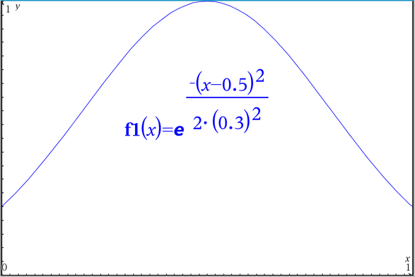
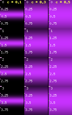
This formula produces a figure that sort of looks like a hill. It peaks in the middle and fades smoothly to the sides. This hill represents the brightness of each scanline, as a function of distance from its beginning. Plotted in a graphing calculator, it looks like this. The c constant controls how steep that hill is. A small value like 0.1 produces a very narrow hill with very sharp and narrow scanlines, and bigger values produce flatter hills and less pronounced scanlines. 0.3 looked like a good compromise.
This simulates the electron gun passing through in horizontal lines called scanlines, as it renders the picture line by line.
You can download the source code of the right-hand-side illustration in img/coppers.php.
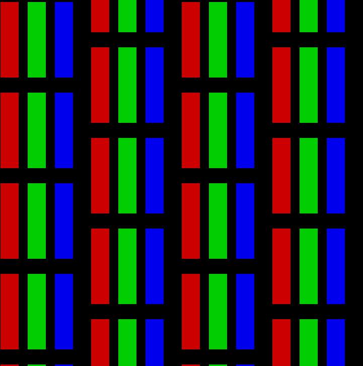
Each color channel and each pixel of the picture — now intermediate width and height — is multiplied by a mask that is either one or zero, depending on whether that pixel belongs inside a cell of that color according to the hardcoded cell geometry.
The mask is a repeating pattern that essentially looks like this:
Red pixels denote 1 for red channel, green pixels denote 1 for green channel, blue pixels denote 1 for blue channel, and everything else for everyone is 0.
This simulates the shadow mask in front of the cathode ray tube.
The mask is generated procedurally from the cell parameters (see Constants).
Then the image is rescaled to the target picture width and target picture height using a Lanczos filter. The scaling is performed first vertically and the horizontally.
A Lanczos filter was chosen because it is generally deemed the best compromise between blurring and fringing among several simple filters (Wikipedia). I have been using it for years for interpolating all sorts of signals from pictures to sounds.
First, the brightness of each pixel is normalized so that the sum of masks and scanline magnitudes does not change the overall brightness of the picture.
Then, a copy is created of the picture. This copy is gamma-corrected and amplified with a significant factor, to promote bloom.
This copy is 2D-gaussian-blurred using a three-step box filter, where the blur width is set as output-width / 640. The blur algorithm is very fast and works in linear time, adapted from http://blog.ivank.net/fastest-gaussian-blur.html .
Then, the actual picture is gamma-corrected, this time without a brightening factor.
Then, the blurry copy is merged into the picture, by literally adding its pixel values into the target pixel values.
Because of the combination of amplification and blurring, if there are isolated bright pixels in the scene, their power is spread out on big area and thus do not contribute much to the final picture, but if there is a large cluster of bright pixels closeby, they remain bright even after blurring, and will influence the final picture a lot. This produces a bloom effect.
Finally, before quantizing the floating-point colors and sending the frame to output, each pixel is clamped to the target range using a desaturation formula.
The desaturation formula first calculates a luminosity value from the input R,G,B components using ITU coefficients (see sRGB on Wikipedia):
- If the luminosity is less than 0, black is returned.
- If the luminosity is more than 1, white is returned.
- Otherwise, a saturation value is initialized as 1, and then adjusted by inspecting each color channel value separately:
After analyzing all color channels, if the saturation still remains as 1, the input color is returned verbatim. Otherwise each color channel is readjusted as:
The readjusted color channel values are then joined together to form the returned color.
The advantage of desaturation-aware clamping over naïve clamping is that it does a much better job at preserving energy. To illustrate, here is a picture with two color ramps. The brightness of the color ramp increases linearly along the Y axis. That is, top is darkest (0) and bottom is brightest (1, i.e. full). Every pixel on each scanline should be approximately same brightness.
The brightness scaling in this illustration is done by simply multiplying the RGB color with the brightness value. At high brightness values, this produces colors that are impossible to show on the screen.
In the leftside picture with naïve clamping (i.e. if x>255, then set x to 255),
you can see that the further
down you go in the picture, the more different the color brightnesses are.
The blue stripe is much, much darker than anything else in the picture,
even though it is fully saturated and as bright as your screen can make it.*
However, on the right side, with the desaturation aware clamping formula, every scanline remains at perfectly even brightness, even when you exceed the maximum possible brightness of the screen colors.
In the desaturation-aware algorithm, colors that are impossible to show on screen due to excess brightness are approximated with desaturated versions, that preserve the brightness perception at the cost of color saturation.
(Note: “Perfectly” was a hyperbole. The colors are not quite the same brightness, because of differences in screen calibration and because of differences in human individual eyes. This is more of an illustration.) You can download the source code of this illustration in img/rainbow.php.
Note that this does not mean that all colors become more washed out. You may come to this mistaken conclusion, because this illustration is fixed for perceptual brightness. The only colors that will be desaturated are those that are have out-of-range values (i.e. individual channel values are greater than 255 or smaller than 0); marked with crosshatch pattern in the below picture. Everything else is kept unchanged.
*) Note that #0000FF is not blue at brightness 1. While it is maximally bright fully saturated blue, its brightness is only about 10 % of the brightness of #00FF00, maximally bright fully saturated green, and only about 7 % of the brightness of #FFFFFF, a maximally bright white pixel (which does have brightness level of 1).
This is trivial to prove: #FFFFFF is a color where you light up all the LEDs that comprise color #0000FF, but you also light up all the LEDs that comprise #FF0000 and all the LEDs that comprise #00FF00. Because there are three times as many LEDs shining as when just #0000FF is shown, the brightness of #FFFFFF cannot be the same, but has to be much higher. Therefore, #0000FF cannot have brightness level of 1.
It is also worth noting that brightness is not the same as radiant energy. This has nothing to do with energy. The human eye is simply differently sensitive to different wavelengths of visible light; least of them to blue (see V(λ)). Brightness is a perception phenomenon.
