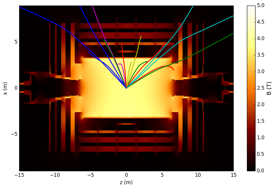
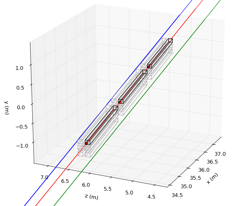
A general-purpose particle trajectory simulator that can propagate a particle through a magnetic field, implement basic multiple scattering and Bethe-Bloch energy loss, and generate statistics on the intersections of these trajectories with an exernal plane (e.g., the Milliqan detector).
Note on units and coordinates: throughout the software, units used are meters for distance, MeV for mass/momentum/energy, nanoseconds for time, and electron-charge units for charge. Coordinates used are CMS coordinates, with the beamline being the z direction.
The package is entirely written in Python (v 2.7 should now run in 2.7 and 3.x). The only absolute requirement is the numpy
library. Optional but useful are the matplotlib library to make plots, pyROOT to get input
from or output to a ROOT file, and numba if you want to use the fast_integrate module to get
a ~100x speed up.
To setup, run . setup.sh from the main directory. This will properly set your PYTHONPATH environment variable
and check for the required packages.
To run a simple check that everything is working, you can go to the test directory and run python validate_helix.py.
This will propagate a particle through a uniform magnetic field and compare the trajectory with the expected helix.
You should see a plot of the x and y coorinates as a function of time.
More advanced tests are in test/functionality_tests.py. This will run through a few examples with muons
to test b-field propagation, multiple scattering, and Bethe-Bloch energy loss and visualize the results.
The millisim directory is a python module with 5 submodules, which are imported into a user-written main script.
Examples of their use are in test/functionality_tests.py.
- Environment.py - implements an
Environmentclass that stores b-field/material configuration. Also contains constants defining material properties. - Integrator.py - implements an
Integratorclass that controls the propagation of particles through a givenEnvironment - Detector.py - contains classes implementing "Detectors". These take a trajectory as input and return information about the interaction of the particle
with the detector. E.g., the location and direction of a particle upon intersection with a detector face. There is a simple
PlaneDetector, which simply detects intersections of trajectories with a rectangle, and a more complicatedMilliqanDetectorthat implements a full 3D bars layout, and can determine which bars a given trajectory hits. - MatterInteractions.py - methods implementing multiple scattering and Bethe-Bloch energy loss (used internally, probably don't need to touch in user script)
- Drawing.py - various methods to make plots of trajectories
The test directory contains a few well-commented example scripts that should give a good idea of how to use the program. In addition
to the test scripts mentioned above, milliqan_test.py is a program to simulate particle hits (muons or mCPs) on a pseudo Milliqan detector (enlarged for demonstration purposes). This also shows how to retrieve information on the intersection of a trajectory with the Milliqan bars.
The bfield directory contains the pickled-version of the CMS magnetic field map. This is loaded into memory at the start
of the simulation. There is also a script to make a 2D plot of the field.
The p_eta_dist directory contains a sample root file with pT and eta distributions of hypothetical milli-charged particles.
This is used by test/milliqan_test.py to generate the initial kinematics of these particles.
For out-of-the-box use, you shouldn't have to edit any of the files in the millisim directory. Everything can be controlled from
the user-written main script. A few examples of these are in the test directory. You should start each script by defining an Environment
(with desired B-field and material setup), and then an Integrator that will propagate particles through this environment.
Configurable parameters for these classes are listed below:
Environment parameters:
bfield: one of["none", "uniform", "updown", "cms"]."uniform"is a uniform 1 T field in the +z direction."cms"will load the CMS magnetic field map defined in the file provided to the next argumentbfield_file: the pickled file of arrays containg the CMS magentic field. Required ifbfield = "cms"above. The map is located inbfield/bfield_coarse.pkl.mat_setup: one of["none", "sife", "cms"], or"unif_"+mat_name, wheremat_nameis any of the defined materials (for a uniform material)."cms"is a very simplified model of CMS.interpolate_b: whether to interpolate B-field values, or just use closest defined point (defaultTrue).use_fine_bfield: configure to use a fine-binned B-field (used in the past, probably never needed anymore)rock_begins: If usingmat_setup = "cms", this is the distance from the origin where a uniform"rock"material is assumed.
Integrator parameters:
environ: an Environment class object through which to propagate particlem,Q: the mass and charge of the particle to propagatedt, nsteps: timestep (in ns) and maximum number of steps to simulatecutoff_dist: stop propagation early once it reaches this distancecutoff_axis: how to measure this distance.'x','y','z'for the x, y, z coordinates.'r'forsrqt(x^2+y2).'R'forsqrt(x^2+y^2+z^2)multiple_scatter: algorithm to use for multiple scattering. Can be one of['none', 'pdg', 'kuhn']('pdg'is simple small-angle gaussian scattering described in this PDG chapter.'kuhn'is a more advanced algorithm that has more realistic, larger tails in the scattering angle distribution ("Rutherford scattering"). Probably not necessary).do_energy_loss: simulate dE/dx energy lossuse_var_dt: if this isTrue, then use a variable dt when velocity is low (when momentum < mass)lowv_dx: if use_var_dt is set, this is the fixed spatial displacement to use when recomputing dt (in m)update func: if you want to specify a custom update function that computes dx/dt at each timesteprandomize_charge_sign: everytime 'propagate' is called, randomly flip sign of Q
You can also define a Detector object that will take a computed trajectory and return information. Currently the only
one implemented is PlaneDetector, which is a rectangular plane with normal vector pointing at the origin.
PlaneDetector parameters:
dist_to_origin: the distance from the face of the detector to the origineta, phi: the eta/phi of the center of detector facewidth, height: the dimensions of rectagular. If either or both areNone, that dimension is infinite
MilliqanDetector parameters:
dist_to_origin: the distance from the center of the near face of the detector to the origineta, phi: the eta/phi of the center of detector facenrows, ncols: number of rows/cols of bars in each layerbar_width, bar_height, bar_length: dimensions of barsbar_gap: gap between bars within a single layerlayer_gap: gap between layers
Once you've defined everything, you can call the Integrator.propagate method to compute a particle trajectory. This implements a Runge-Kutta integrator
that will propagate a particle through the magnetic field, and simulates multiple scattering/energy loss if these are turned on.
The only argument is a 6-element vector x0 that contains the initial position and momentum [x, y, z, px, py, pz] (as always, position is in meters and momentum in MeV).
At each timestep, the function Integrator.update_func is called (defaults to Integrator.dxdt_bfield) that computes dx/dt given the current time/position/momentum.
This is used to update the 6-element x vector. The change in position/momentum are modified to account for multiple scattering and energy loss if turned on
(multiple scattering is a random process, energy loss is deterministic).
The return value of Integrator.propagate is a 6-by-(nsteps+1) array. Each column contains [x,y,z,px,py,pz] at a specific timestep.
The PlaneDetector.find_intersection method takes the trajectory array defined above and computes statistics on the intersection with
an external plane, and returns a dictionary of useful values. MilliqanDetector.find_entries_exits returns the entry and exit points of a given trajectory for each bar it passes through. See millisim/Detector.py and test/milliqan_test.py for details.

