PreTrends

The pretrends package provides tools for power calculations for pre-trends tests, and visualization of possible violations of parallel trends. Calculations are based on Roth (2022). This is the Stata version of the R package of the same name. (Please cite the paper if you enjoy the package!)

If you’re not an R or Stata user, you may also be interested in the associated Shiny app.

version 0.3.1 20Mar2023 | Installation | Application

Installation

The package may be installed by using net install:

local github https://raw.githubusercontent.com
net install pretrends, from(`github'/mcaceresb/stata-pretrends/main) replace

You can also clone or download the code manually, e.g. to stata-pretrends-main, and install from a local folder:

cap noi net uninstall pretrends
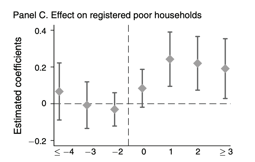
net install pretrends, from(`c(pwd)'/stata-pretrends-main)

Application to He and Wang (2017)

We illustrate how to use the package with an application to He and Wang (2017). The analysis will be based on the event-study in Figure 2C, which looks like this:

Load the example data

Next we load the estimation results used for the event-plot, namely the coefficients (beta), the variance-covariance matrix (sigma). In this case, these coefficients come from a two-way fixed effects regression, but the pretrends package can accommodate an event-study from any asymptotically normal estimator, including Callaway and Sant’Anna (2020) and Sun and Abraham (2020).

mata {
    st_matrix("beta",  PreTrendsExampleBeta())
    st_matrix("sigma", PreTrendsExampleSigma())
}
matlist beta'
*              |        r1
* -------------+----------
*           c1 |  .0667031
*           c2 | -.0077018
*           c3 | -.0307691
*           c4 |  .0840307
*           c5 |  .2424418
*           c6 |   .219879
*           c7 |  .1910925

Using the package

First, the user must specify the coefficient vector, variance-covariance matrix, and the sections therein that correspond to the pre and post periods. By default, the package tries to use e(b) and e(V), which would be populated after most estimation commands.

Second, the user has two options:

1. The power sub-command calculates the slope of a linear violation of parallel trends that a pre-trends test would detect a specified fraction of the time. (By detect, we mean that there is any significant pre-treatment coefficient.)

2. Alternatively, the user can specify a hypothesized violations of parallel trends --- the package then creates a plot to visualize the results, and reports various statistics related to the hypothesized difference in trend. The user can specify a hypothesized linear pre-trend via the slope() option, or provide an arbitrary violation of parallel trends via the delta() option.

Let's illustrate the first use case:

pretrends power 0.5, numpre(3) b(beta) v(sigma)
* Slope for 50% power =  .0520662

return list
* scalars:
*               r(slope) =  .0520662478209672
*               r(Power) =  .5

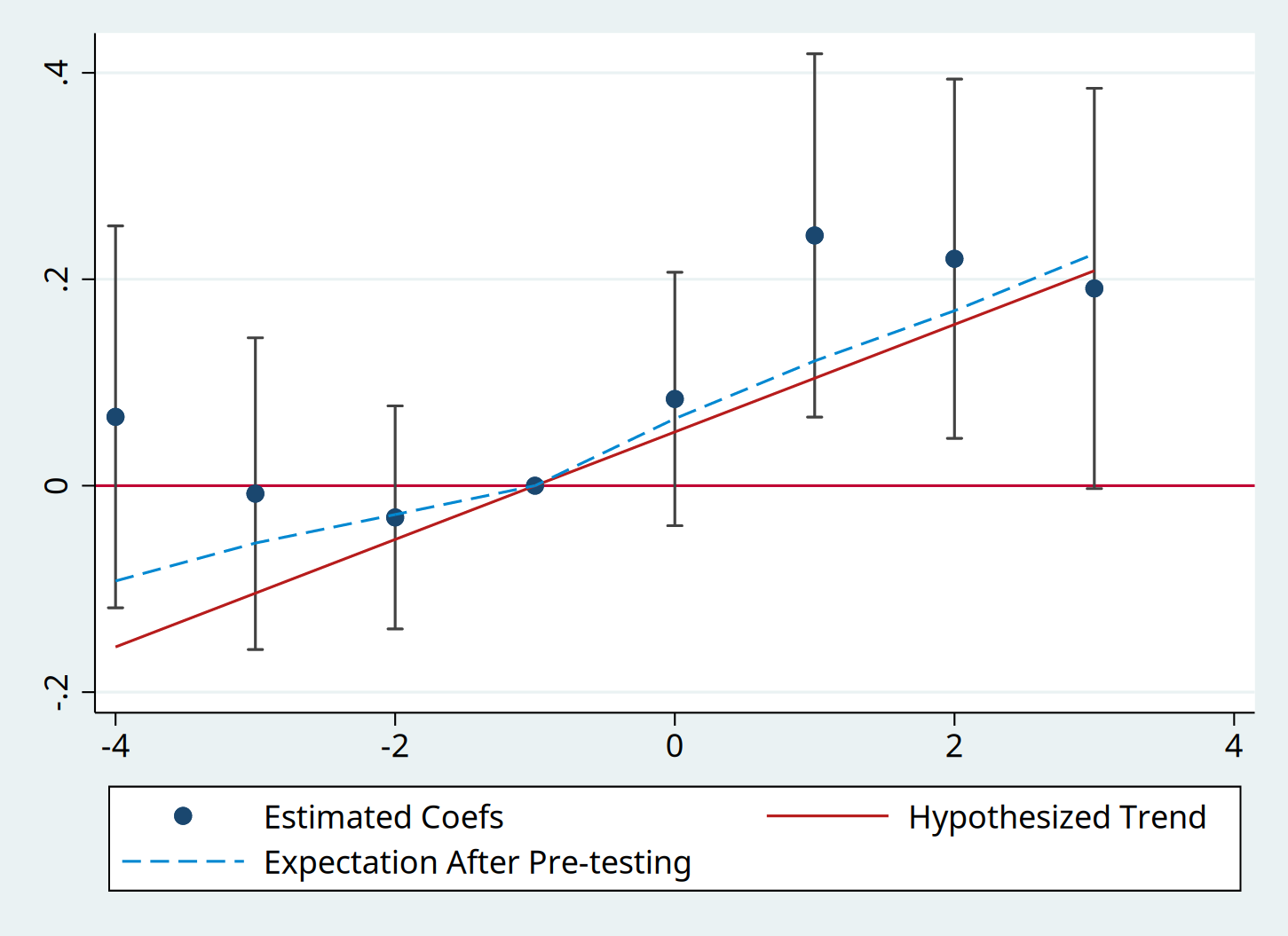
To visualize the linear trend against which pre-tests have 50 percent power:

pretrends, numpre(3) b(beta) v(sigma) slope(`r(slope)')

Note the coefplot package is required; if the coefplot package is not installed or not available, the user can add option nocoefplot to skip the visualization. In either case the event study data is saved in r(), along several useful statistics about the power of the pre-test against the hypothesized trend.

* data for visualization
matlist r(results)
*              |         t    betahat         lb         ub  deltatrue  meanAft~g
* -------------+------------------------------------------------------------------
*           r1 |        -4   .0667031  -.1182677    .251674  -.1561987  -.0923171
*           r2 |        -3  -.0077018  -.1587197   .1433162  -.1041325  -.0555576
*           r3 |        -2  -.0307691  -.1388096   .0772715  -.0520662  -.0279117
*           r4 |        -1          0          0          0          0          0
*           r5 |         0   .0840307  -.0387567    .206818   .0520662   .0649147
*           r6 |         1   .2424418   .0664168   .4184668   .1041325   .1208691
*           r7 |         2    .219879   .0458768   .3938812   .1561987   .1694932
*           r8 |         3   .1910925  -.0028194   .3850045    .208265   .2245753

return list
* scalars:
*                  r(LR) =  .1057053243787036
*               r(Bayes) =  .5690176871738699
*               r(Power) =  .5000000000006959
*               r(slope) =  .0520662478209672
*
* macros:
*    r(PreTrendsResults) : "PreTrendsResults"
*
* matrices:
*             r(results) :  8 x 6
*               r(delta) :  1 x 8

• r(results) The data used to make the event plot. Note the column meanAfterPretesting, which is also plotted, shows the expected value of the coefficients conditional on passing the pre-test under the hypothesized trend.

• r(Power) The probability that we would find a significant pre-trend under the hypothesized pre-trend. (This is 0.50, up to numerical precision error, by construction in our example).

• r(BF) (Bayes Factor) The ratio of the probability of "passing" the pre-test under the hypothesized trend relative to under parallel trends.

• r(LR) (Likelihood Ratio) The ratio of the likelihood of the observed coefficients under the hypothesized trend relative to under parallel trends.

The package can also compute the above in one step:

pretrends, numpre(3) b(beta) v(sigma) power(0.5) nocoefplot
matlist r(results)
return list

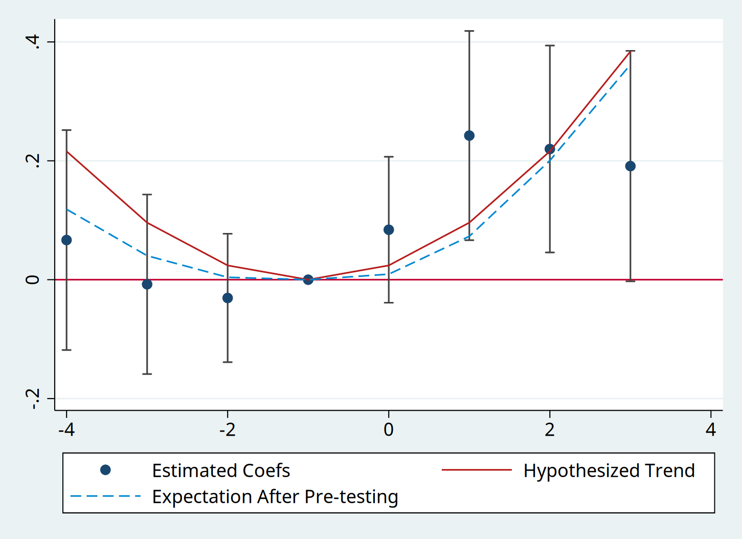
Last, although our example has focused on a linear violation of parallel trends, the package allows the user to input an arbitrary non-linear hypothesized trend. For instance, here is the event-plot and power analysis from a quadratic trend.

mata st_matrix("deltaquad", 0.024 * ((-4::3) :- (-1)):^2)
pretrends, numpre(3) b(beta) v(sigma) deltatrue(deltaquad) coefplot

matlist r(results)
*              |         t    betahat         lb         ub  deltatrue  meanAft~g
* -------------+------------------------------------------------------------------
*           r1 |        -4   .0667031  -.1182677    .251674       .216   .1184861
*           r2 |        -3  -.0077018  -.1587197   .1433162       .096    .040358
*           r3 |        -2  -.0307691  -.1388096   .0772715       .024   .0040393
*           r4 |        -1          0          0          0          0          0
*           r5 |         0   .0840307  -.0387567    .206818       .024   .0093079
*           r6 |         1   .2424418   .0664168   .4184668       .096    .072993
*           r7 |         2    .219879   .0458768   .3938812       .216   .2004382
*           r8 |         3   .1910925  -.0028194   .3850045       .384   .3617779

return list
* scalars:
*                  r(LR) =  .4332635208743188
*               r(Bayes) =  .3841447004284795
*               r(Power) =  .6624492444726371
*               r(slope) =  .
*
* macros:
*    r(PreTrendsResults) : "PreTrendsResults"
*
* matrices:
*             r(results) :  8 x 6
*               r(delta) :  1 x 8