bpf4 is a python library to operate with curves in 2D space.
Curves can be defined via breakpoints (break-point functions, hence the name) or using functions. Moreover, curves can be used to build other curves. bpf4 can be used to perform curve fitting, data analysis, plotting, etc. Its core is programmed in cython for efficiency.
pip install --upgrade bpf4
The documentation is hosted at https://bpf4.readthedocs.io
Find the intersection between two curves
from bpf4 import bpf  # this imports the api
a = bpf.spline((0, 0), (1, 5), (2, 3), (5, 10))  # each point (x, y)
b = bpf.expon((0, -10), (2,15), (5, 3), exp=3)
a.plot() # uses matplotlib
b.plot()
zeros = (a - b).zeros()
import pylab
pylab.plot(zeros, a.map(zeros), 'o')Many interpolation types besides linear:
- spline
- univariate splie
- pchip (hermite)
- cosine
- exponential
- logarithmic
- etc.
With the exception of curve-fitting bpfs (splines), interpolation types can be mixed, so that each segment has a different interpolation. Following from the example above:
c = (a + b).sin().abs()
# plot only the range (1.5, 4)
c[1.5:4].plot()
Syntax support for shifting, scaling and slicing a bpf
a >> 2        # a shifted to the right
(a * 5) ^ 2   # scale the x coord by 2, scale the y coord by 5
a[2:2.5]      # slice only a portion of the bpf
a[::0.01] # sample the bpf with an interval of 0.01from bpf4 import *
a = spline((0, 0), (1, 5), (2, 3), (5, 10))
deriv = a.derivative()
integr = a.integrated()
import matplotlib.pyplot as plt
fig, axs = plt.subplots(3, 1, sharex=True, figsize=(16, 8), tight_layout=True)
a.plot(axes=axs[0], show=False)
deriv.plot(axes=axs[1], show=False)
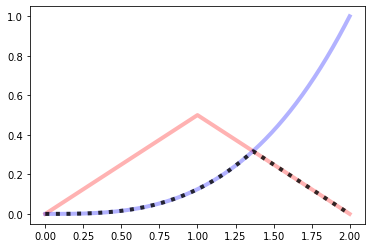
integr.plot(axes=axs[2])a = linear(0, 0, 1, 0.5, 2, 0)
b = expon(0, 0, 2, 1, exp=3)
a.plot(show=False, color="red", linewidth=4, alpha=0.3)
b.plot(show=False, color="blue", linewidth=4, alpha=0.3)
core.Max((a, b)).plot(color="black", linewidth=4, alpha=0.8, linestyle='dotted')a = linear(0, 0, 1, 0.5, 2, 0)
b = expon(0, 0, 2, 1, exp=3)
a.plot(show=False, color="red", linewidth=4, alpha=0.3)
b.plot(show=False, color="blue", linewidth=4, alpha=0.3)
core.Min((a, b)).plot(color="black", linewidth=4, alpha=0.8, linestyle='dotted')a = linear(0, 0, 1, 0.5, 2, 0)
b = expon(0, 0, 2, 1, exp=3)
a.plot(show=False, color="red", linewidth=4, alpha=0.3)
b.plot(show=False, color="blue", linewidth=4, alpha=0.3)
(a*b).plot(color="black", linewidth=4, alpha=0.8, linestyle='dotted')
a = linear(0, 0, 1, 0.5, 2, 0)
b = expon(0, 0, 2, 1, exp=3)
a.plot(show=False, color="red", linewidth=4, alpha=0.3)
b.plot(show=False, color="blue", linewidth=4, alpha=0.3)
(a**b).plot(color="black", linewidth=4, alpha=0.8, linestyle='dotted')
a = linear(0, 0, 1, 0.5, 2, 0)
b = expon(0, 0, 2, 1, exp=3)
a.plot(show=False, color="red", linewidth=4, alpha=0.3)
b.plot(show=False, color="blue", linewidth=4, alpha=0.3)
((a+b)/2).plot(color="black", linewidth=4, alpha=0.8, linestyle='dotted')A bpf can be used to build complex formulas
Fresnel's Integral: ( S(x) = \int_0^x {sin(t^2)} dt )
t = slope(1)
f = (t**2).sin()[0:10:0.001].integrated()
f.plot()Any kind of matplotlib plot can be used. For example, polar plots are possible
by creating an axes with polar=True
Cardiod: (\rho = 1 + sin(-\theta) )
from math import *
theta = slope(1, bounds=(0, 2*pi))
r = 1 + (-theta).sin()

ax = plt.axes(polar=True)
ax.set_rticks([0.5, 1, 1.5, 2]); ax.set_rlabel_position(38)
r.plot(axes=ax)
Flower 5: (\rho = 3 + cos(5 * \theta) )
theta = core.Slope(1, bounds=(0, 2*pi))
r = 3 + (5*theta).cos()

ax = plt.axes(polar=True)
r.plot(axes=ax)


