##Preface
This is a hands-on guide to machine learning for programmers with no background in AI. Using a neural network doesn’t require a PhD, and you don’t need to be the person who makes the next breakthrough in AI in order to use what exists today. What we have now is already breathtaking, and highly usable. I believe that more of us need to play with this stuff like we would any other open source technology, instead of treating it like a research topic.
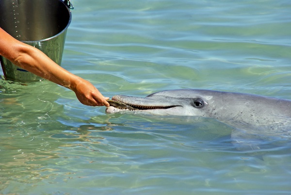
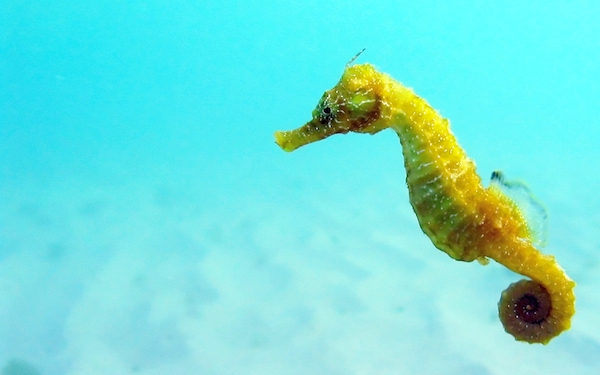
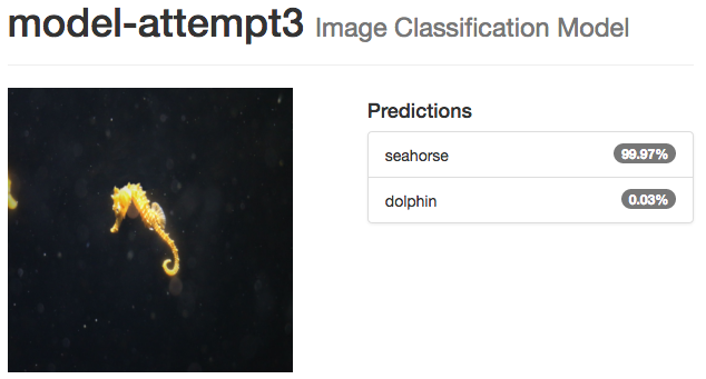
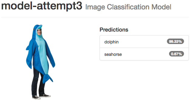
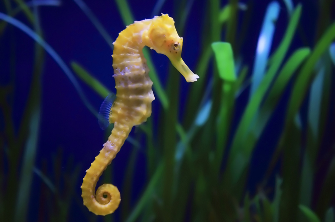
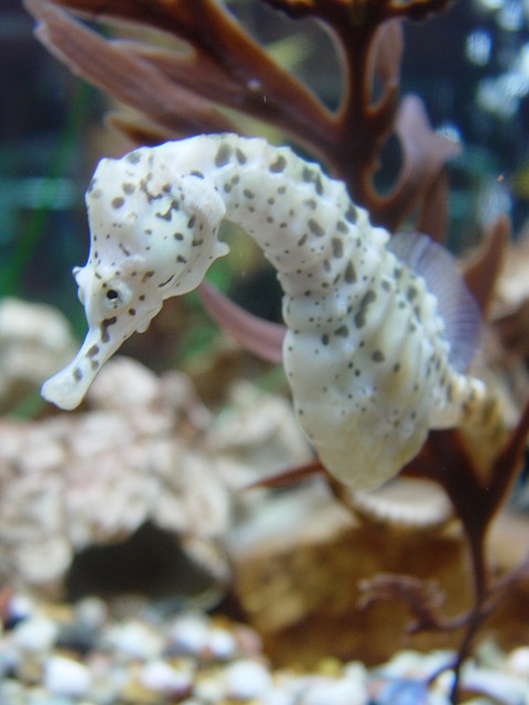
In this guide our goal will be to write a program that uses machine learning to predict, with a high degree of certainty, whether the images in data/untrained-samples are of dolphins or seahorses using only the images themselves, and without having seen them before. Here are two example images we'll use:
To do that we’re going to train and use a Convolutional Neural Network (CNN). We’re going to approach this from the point of view of a practitioner vs. from first principles. There is so much excitement about AI right now, but much of what’s being written feels like being taught to do tricks on your bike by a physics professor at a chalkboard instead of your friends in the park.
I’ve decided to write this on Github vs. as a blog post because I’m sure that some of what I’ve written below is misleading, naive, or just plain wrong. I’m still learning myself, and I’ve found the lack of solid beginner documentation an obstacle. If you see me making a mistake or missing important details, please send a pull request.
With all of that out the way, let me show you how to do some tricks on your bike!
##Overview
Here’s what we’re going to explore:
- Setup and use existing, open source machine learning technologies, specifically Caffe and DIGITS
- Create a dataset of images
- Train a neural network from scratch
- Test our neural network on images it has never seen before
- Improve our neural network’s accuracy by fine tuning existing neural networks (AlexNet and GoogLeNet)
- Deploy and use our neural network
This guide won’t teach you how neural networks are designed, cover much theory, or use a single mathematical expression. I don’t pretend to understand most of what I’m going to show you. Instead, we’re going to use existing things in interesting ways to solve a hard problem.
Q: "I know you said we won’t talk about the theory of neural networks, but I’m feeling like I’d at least like an overview before we get going. Where should I start?"
There are literally hundreds of introductions to this, from short posts to full online courses. Depending on how you like to learn, here are three options for a good starting point:
- This fantastic blog post by J Alammar, which introduces the concepts of neural networks using intuitive examples.
- Similarly, this video introduction by Brandon Rohrer is a really good intro to Convolutional Neural Networks like we'll be using
- If you’d rather have a bit more theory, I’d recommend this online book by Michael Nielsen.
##Setup
###Installing Caffe
First, we’re going to be using the Caffe deep learning framework from the Berkely Vision and Learning Center (BSD licensed).
Q: “Wait a minute, why Caffe? Why not use something like TensorFlow, which everyone is talking about these days…”
There are a lot of great choices available, and you should look at all the options. TensorFlow is great, and you should play with it. However, I’m using Caffe for a number of reasons:
- It’s tailormade for computer vision problems
- It has support for C++, Python, (with node.js support coming)
- It’s fast and stable
But the number one reason I’m using Caffe is that you don’t need to write any code to work with it. You can do everything declaratively (Caffe uses structured text files to define the network architecture) and using command-line tools. Also, you can use some nice front-ends for Caffe to make training and validating your network a lot easier. We’ll be using nVidia’s DIGITS tool below for just this purpose.
Caffe can be a bit of work to get installed. There are installation instructions for various platforms, including some prebuilt Docker or AWS configurations.
NOTE: when making my walkthrough, I used the following non-released version of Caffe from their Github repo: https://github.com/BVLC/caffe/commit/5a201dd960840c319cefd9fa9e2a40d2c76ddd73
On a Mac it can be frustrating to get working, with version issues halting your progress at various steps in the build. It took me a couple of days of trial and error. There are a dozen guides I followed, each with slightly different problems. In the end I found this one to be the closest. I’d also recommend this post, which is quite recent and links to many of the same discussions I saw.
Getting Caffe installed is by far the hardest thing we'll do, which is pretty neat, since you’d assume the AI aspects would be harder! Don’t give up if you have issues, it’s worth the pain. If I was doing this again, I’d probably use an Ubuntu VM instead of trying to do it on Mac directly. There's also a Caffe Users group, if you need answers.
Q: “Do I need powerful hardware to train a neural network? What if I don’t have access to fancy GPUs?”
It’s true, deep neural networks require a lot of computing power and energy to train...if you’re training them from scratch and using massive datasets. We aren’t going to do that. The secret is to use a pretrained network that someone else has already invested hundreds of hours of compute time training, and then to fine tune it to your particular dataset. We’ll look at how to do this below, but suffice it to say that everything I’m going to show you, I’m doing on a year old MacBook Pro without a fancy GPU.
As an aside, because I have an integrated Intel graphics card vs. an nVidia GPU, I decided to use the OpenCL Caffe branch, and it’s worked great on my laptop.
When you’re done installing Caffe, you should have, or be able to do all of the following:
- A directory that contains your built caffe. If you did this in the standard way,
there will be a
build/dir which contains everything you need to run caffe, the Python bindings, etc. The parent dir that containsbuild/will be yourCAFFE_ROOT(we’ll need this later). - Running
make test && make runtestshould pass - After installing all the Python deps (doing
for req in $(cat requirements.txt); do pip install $req; doneinpython/), runningmake pycaffe && make pytestshould pass - You should also run
make distributein order to create a distributable version of caffe with all necessary headers, binaries, etc. indistribute/.
On my machine, with Caffe fully built, I’ve got the following basic layout in my CAFFE_ROOT dir:
caffe/
    build/
        python/
        lib/
        tools/
            caffe ← this is our main binary
    distribute/
        python/
        lib/
        include/
        bin/
        proto/
At this point, we have everything we need to train, test, and program with neural networks. In the next section we’ll add a user-friendly, web-based front end to Caffe called DIGITS, which will make training and testing our networks much easier.
###Installing DIGITS
nVidia’s Deep Learning GPU Training System, or DIGITS, is BSD-licensed Python web app for training neural networks. While it’s possible to do everything DIGITS does in Caffe at the command-line, or with code, using DIGITS makes it a lot easier to get started. I also found it more fun, due to the great visualizations, real-time charts, and other graphical features. Since you’re experimenting and trying to learn, I highly recommend beginning with DIGITS.
There are quite a few good docs at https://github.com/NVIDIA/DIGITS/tree/master/docs, including a few Installation, Configuration, and Getting Started pages. I’d recommend reading through everything there before you continue, as I’m not an expert on everything you can do with DIGITS. There's also a public DIGITS User Group if you have questions you need to ask.
There are various ways to install and run DIGITS, from Docker to pre-baked packages on Linux, or you can build it from source. I’m on a Mac, so I built it from source.
NOTE: In my walkthrough I've used the following non-released version of DIGITS from their Github repo: https://github.com/NVIDIA/DIGITS/commit/81be5131821ade454eb47352477015d7c09753d9
Because it’s just a bunch of Python scripts, it was fairly painless to get working.
The one thing you need to do is tell DIGITS where your CAFFE_ROOT is by setting
an environment variable before starting the server:
export CAFFE_ROOT=/path/to/caffe
./digits-devserver
NOTE: on Mac I had issues with the server scripts assuming my Python binary was
called python2, where I only have python2.7. You can symlink it in /usr/bin
or modify the DIGITS startup script(s) to use the proper binary on your system.
Once the server is started, you can do everything else via your web browser at http://localhost:5000, which is what I'll do below.
##Training a Neural Network
Training a neural network involves a few steps:
- Assemble and prepare a dataset of categorized images
- Define the network’s architecture
- Train and Validate this network using the prepared dataset
We’re going to do this 3 different ways, in order to show the difference between starting from scratch and using a pretrained network, and also to show how to work with two popular pretrained networks (AlexNet, GoogLeNet) that are commonly used with Caffe and DIGITs.
For our training attempts, we’ll use a small dataset of Dolphins and Seahorses. I’ve put the images I used in data/dolphins-and-seahorses. You need at least 2 categories, but could have many more (some of the networks we’ll use were trained on 1000+ image categories). Our goal is to be able to give an image to our network and have it tell us whether it’s a Dolphin or a Seahorse.
###Prepare the Dataset
The easiest way to begin is to divide your images into a categorized directory layout:
dolphins-and-seahorses/
    dolphin/
        image_0001.jpg
        image_0002.jpg
        image_0003.jpg
        ...
    seahorse/
        image_0001.jpg
        image_0002.jpg
        image_0003.jpg
        ...
Here each directory is a category we want to classify, and each image within that category dir an example we’ll use for training and validation.
Q: “Do my images have to be the same size? What about the filenames, do they matter?”
No to both. The images sizes will be normalized before we feed them into the network. We’ll eventually want colour images of 256 x 256 pixels, but DIGITS will crop or squash (we'll squash) our images automatically in a moment. The filenames are irrelevant--it’s only important which category they are contained within.
Q: “Can I do more complex segmentation of my categories?”
Yes. See https://github.com/NVIDIA/DIGITS/blob/digits-4.0/docs/ImageFolderFormat.md.
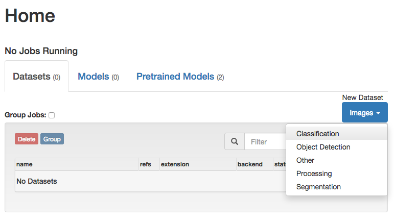
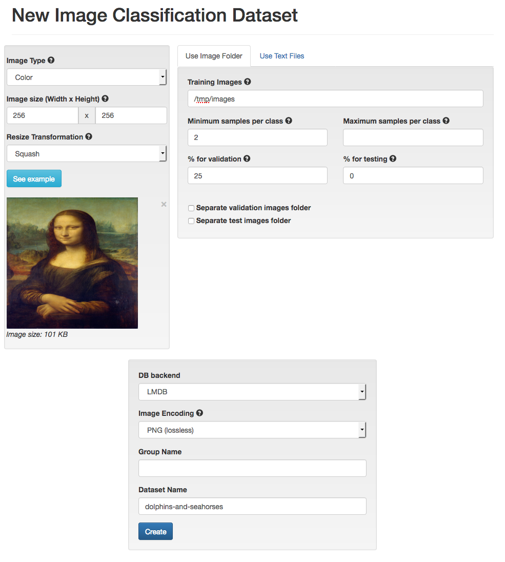
We want to use these images on disk to create a New Dataset, and specifically, a Classification Dataset.
We’ll use the defaults DIGITS gives us, and point Training Images at the path
to our data/dolphins-and-seahorses folder.
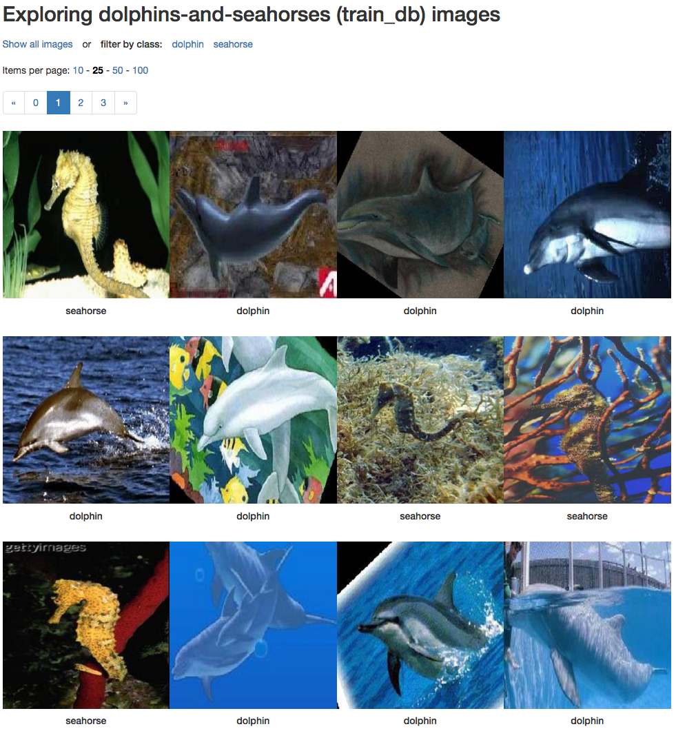
DIGITS will use the categories (dolphin and seahorse) to create a database
of squashed, 256 x 256 Training (75%) and Testing (25%) images.
Give your Dataset a name,dolphins-and-seahorses, and click Create.
This will create our dataset, which took only 4s on my laptop. In the end I have 92 Training images (49 dolphin, 43 seahorse) in 2 categories, with 30 Validation images (16 dolphin, 14 seahorse). It’s a really small dataset, but perfect for our experimentation and learning purposes, because it won’t take forever to train and validate a network that uses it.
You can Explore the db if you want to see the images after they have been squashed.
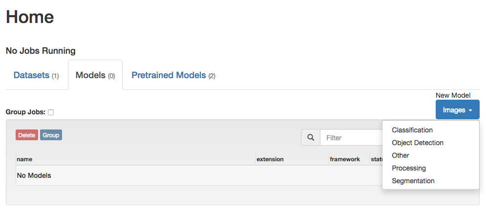
Back in the DIGITS Home screen, we need to create a new Classification Model:
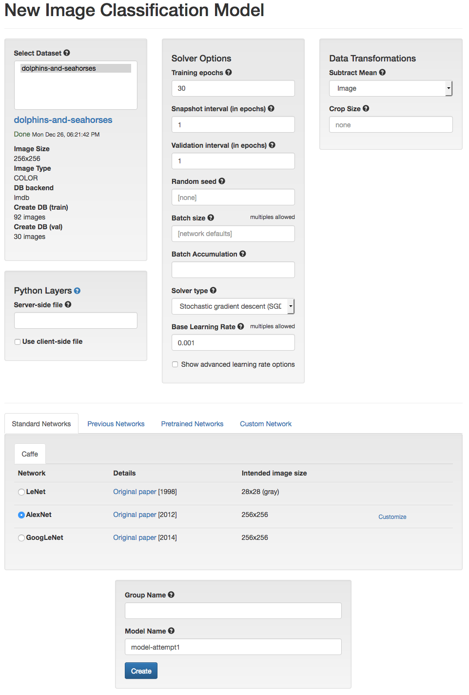
We’ll start by training a model that uses our dolphins-and-seahorses dataset,
and the default settings DIGITS provides. For our first network, we’ll choose to
use one of the standard network architectures, AlexNet (pdf). AlexNet’s design
won a major computer vision competition called ImageNet in 2012. The competition
required categorizing 1000+ image categories across 1.2 million images.
Caffe uses structured text files to define network architectures. These text files are based on Google’s Protocol Buffers. You can read the full schema Caffe uses. For the most part we’re not going to work with these, but it’s good to be aware of their existence, since we’ll have to modify them in later steps. The AlexNet prototxt file looks like this, for example: https://github.com/BVLC/caffe/blob/master/models/bvlc_alexnet/train_val.prototxt.
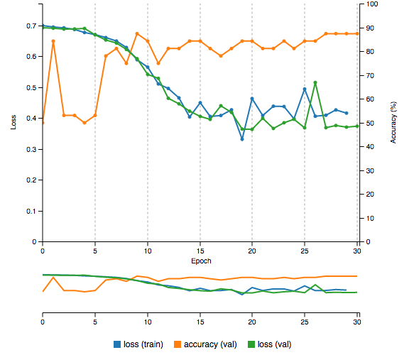
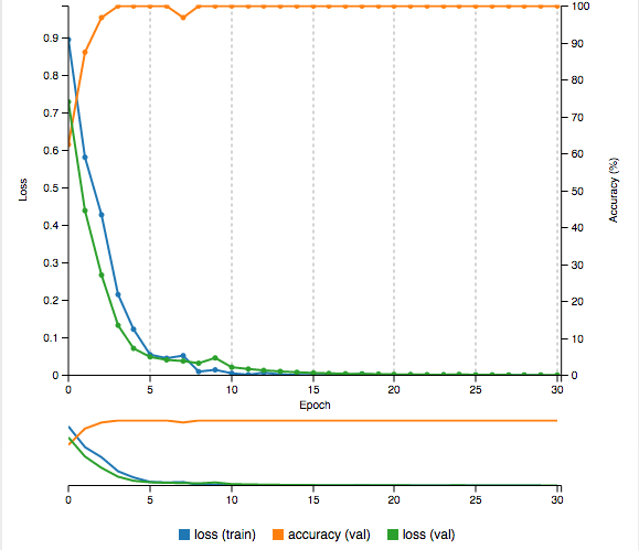
We’ll train our network for 30 epochs, which means that it will learn (with our training images) then test itself (using our validation images), and adjust the network’s weights depending on how well it’s doing, and repeat this process 30 times. Each time it completes a cycle we’ll get info about Accuracy (0% to 100%, where higher is better) and what our Loss is (the sum of all the mistakes that were made, where lower is better). Ideally we want a network that is able to predict with high accuracy, and with few errors (small loss).
Initially, our network’s accuracy is a bit below 50%. This makes sense, because at first it’s just “guessing” between two categories using randomly assigned weights. Over time it’s able to achieve 87.5% accuracy, with a loss of 0.37. The entire 30 epoch run took me just under 6 minutes.
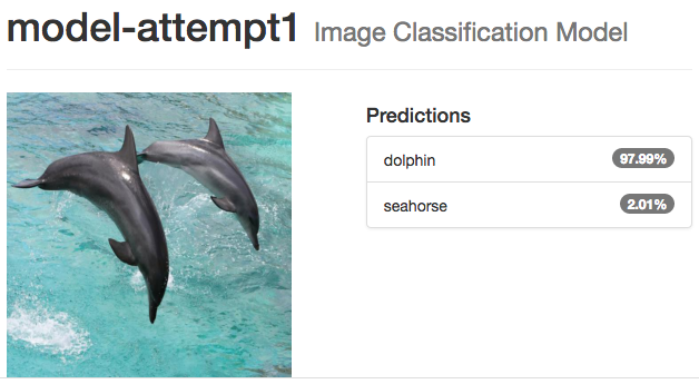
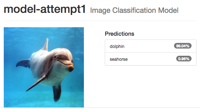
We can test our model using an image we upload or a URL to an image on the web. Let’s test it on a few examples that weren’t in our training/validation dataset:
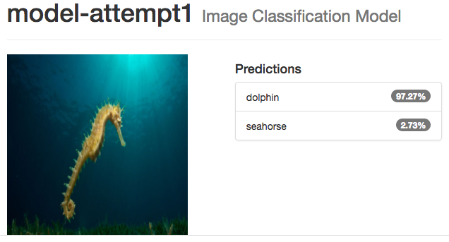
It almost seems perfect, until we try another:
Here it falls down completely, and confuses a seahorse for a dolphin, and worse, does so with a high degree of confidence.
The reality is that our dataset is too small to be useful for training a really good neural network. We really need 10s or 100s of thousands of images, and with that, a lot of computing power to process everything.
####How Fine Tuning works
Designing a neural network from scratch, collecting data sufficient to train it (e.g., millions of images), and accessing GPUs for weeks to complete the training is beyond the reach of most of us. To make it practical for smaller amounts of data to be used, we employ a technique called Transfer Learning, or Fine Tuning. Fine tuning takes advantage of the layout of deep neural networks, and uses pretrained networks to do the hard work of initial object detection.
Imagine using a neural network to be like looking at something far away with a pair of binoculars. You first put the binoculars to your eyes, and everything is blurry. As you adjust the focus, you start to see colours, lines, shapes, and eventually you are able to pick out the shape of a bird, then with some more adjustment you can identify the species of bird.
In a multi-layered network, the initial layers extract features (e.g., edges), with later layers using these features to detect shapes (e.g., a wheel, an eye), which are then feed into final classification layers that detect items based on accumulated characteristics from previous layers (e.g., a cat vs. a dog). A network has to be able to go from pixels to circles to eyes to two eyes placed in a particular orientation, and so on up to being able to finally conclude that an image depicts a cat.
What we’d like to do is to specialize an existing, pretrained network for classifying a new set of image classes instead of the ones on which it was initially trained. Because the network already knows how to “see” features in images, we’d like to retrain it to “see” our particular image types. We don’t need to start from scratch with the majority of the layers--we want to transfer the learning already done in these layers to our new classification task. Unlike our previous attempt, which used random weights, we’ll use the existing weights of the final network in our training. However, we’ll throw away the final classification layer(s) and retrain the network with our image dataset, fine tuning it to our image classes.
For this to work, we need a pretrained network that is similar enough to our own data that the learned weights will be useful. Luckily, the networks we’ll use below were trained on millions of natural images from ImageNet, which is useful across a broad range of classification tasks.
This technique has been used to do interesting things like screening for eye diseases from medical imagery, identifying plankton species from microscopic images collected at sea, to categorizing the artistic style of Flickr images.
Doing this perfectly, like all of machine learning, requires you to understand the data and network architecture--you have to be careful with overfitting of the data, might need to fix some of the layers, might need to insert new layers, etc. However, my experience is that it “Just Works” much of the time, and it’s worth you simply doing an experiment to see what you can achieve using our naive approach.
####Uploading Pretrained Networks
In our first attempt, we used AlexNet’s architecture, but started with random weights in the network’s layers. What we’d like to do is download and use a version of AlexNet that has already been trained on a massive dataset.
Thankfully we can do exactly this. A snapshot of AlexNet is available for download: https://github.com/BVLC/caffe/tree/master/models/bvlc_alexnet.
We need the binary .caffemodel file, which is what contains the trained weights, and it’s
available for download at http://dl.caffe.berkeleyvision.org/bvlc_alexnet.caffemodel.
While you’re downloading pretrained models, let’s get one more at the same time.
In 2014, Google won the same ImageNet competition with GoogLeNet (codenamed Inception):
a 22-layer neural network. A snapshot of GoogLeNet is available for download
as well, see https://github.com/BVLC/caffe/tree/master/models/bvlc_googlenet.
Again, we’ll need the .caffemodel file with all the pretrained weights,
which is available for download at http://dl.caffe.berkeleyvision.org/bvlc_googlenet.caffemodel.
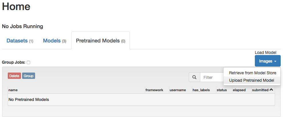
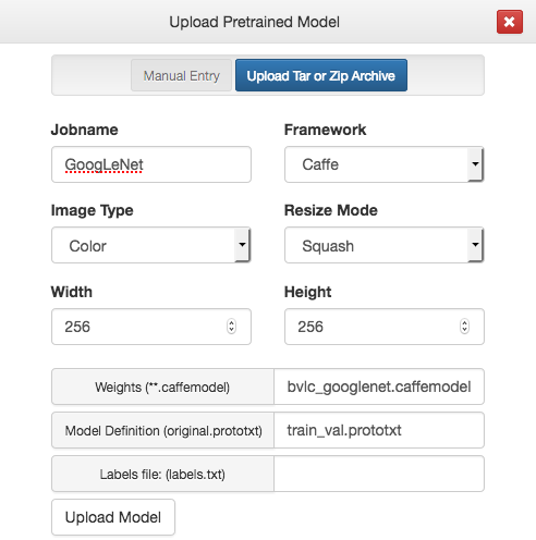
With these .caffemodel files in hand, we can upload them into DIGITs. Go to
the Pretrained Models tab in DIGITs home page and choose Upload Pretrained Model:
For both of these pretrained models, we can use the defaults DIGITs provides
(i.e., colour, squashed images of 256 x 256). We just need to provide the
Weights (**.caffemodel) and Model Definition (original.prototxt).
Click each of those buttons to select a file.
For the model definitions we can use https://github.com/BVLC/caffe/blob/master/models/bvlc_googlenet/train_val.prototxt
for GoogLeNet and https://github.com/BVLC/caffe/blob/master/models/bvlc_alexnet/train_val.prototxt
for AlexNet. We aren’t going to use the classification labels of these networks,
so we’ll skip adding a labels.txt file:
Repeat this process for both AlexNet and GoogLeNet, as we’ll use them both in the coming steps.
Q: "Are there other networks that would be good as a basis for fine tuning?"
The Caffe Model Zoo has quite a few other pretrained networks that could be used, see https://github.com/BVLC/caffe/wiki/Model-Zoo.
####Fine Tuning AlexNet for Dolphins and Seahorses
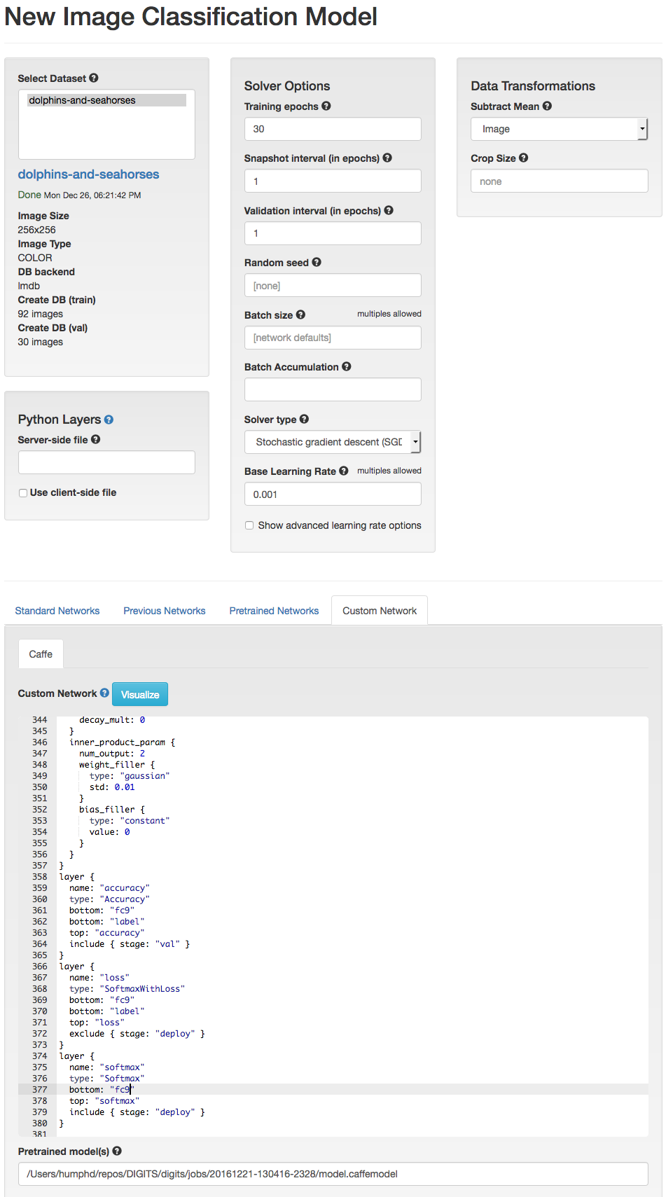
Training a network using a pretrained Caffe Model is similar to starting from scratch, though we have to make a few adjustments. First, we’ll adjust the Base Learning Rate to 0.001 from 0.01, since we don’t need to make such large jumps (i.e., we’re fine tuning). We’ll also use a Pretrained Network, and Customize it.
In the pretrained model’s definition (i.e., prototext), we need to rename all
references to the final Fully Connected Layer (where the end result classifications
happen). We do this because we want the model to re-learn new categories from
our dataset vs. its original training data (i.e., we want to throw away the current
final layer). We have to rename the last fully connected layer from “fc8” to
something else, “fc9” for example. Finally, we also need to adjust the number
of categories from 1000 to 2, by changing num_output to 2.
Here are the changes we need to make:
@@ -332,8 +332,8 @@
 }
 layer {
-  name: "fc8"
+  name: "fc9"
   type: "InnerProduct"
   bottom: "fc7"
-  top: "fc8"
+  top: "fc9"
   param {
     lr_mult: 1
@@ -345,5 +345,5 @@
   }
   inner_product_param {
-    num_output: 1000
+    num_output: 2
     weight_filler {
       type: "gaussian"
@@ -359,5 +359,5 @@
   name: "accuracy"
   type: "Accuracy"
-  bottom: "fc8"
+  bottom: "fc9"
   bottom: "label"
   top: "accuracy"
@@ -367,5 +367,5 @@
   name: "loss"
   type: "SoftmaxWithLoss"
-  bottom: "fc8"
+  bottom: "fc9"
   bottom: "label"
   top: "loss"
@@ -375,5 +375,5 @@
   name: "softmax"
   type: "Softmax"
-  bottom: "fc8"
+  bottom: "fc9"
   top: "softmax"
   include { stage: "deploy" }
I’ve included the fully modified file I’m using in src/alexnet-customized.prototxt.
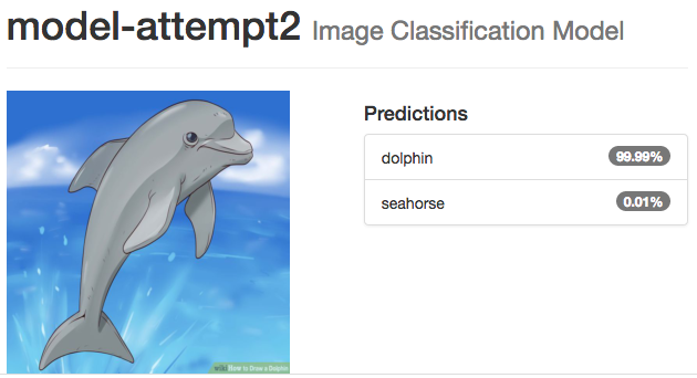
This time our accuracy starts at ~60% and climbs right away to 87.5%, then to 96% and all the way up to 100%, with the Loss steadily decreasing. After 5 minutes we end up with an accuracy of 100% and a loss of 0.0009.
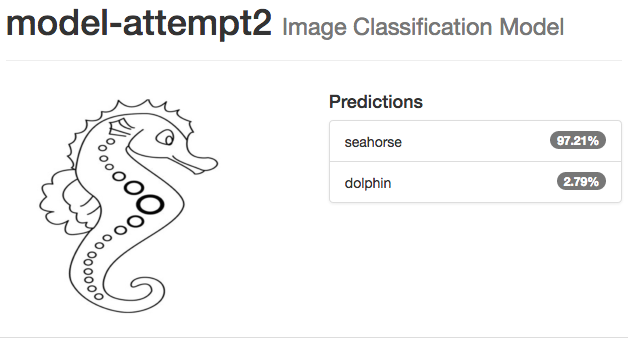
Testing the same seahorse image our previous network got wrong, we see a complete reversal: 100% seahorse.
Even a children’s drawing of a seahorse works:
The same goes for a dolphin:
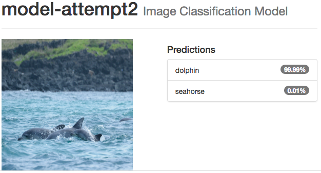
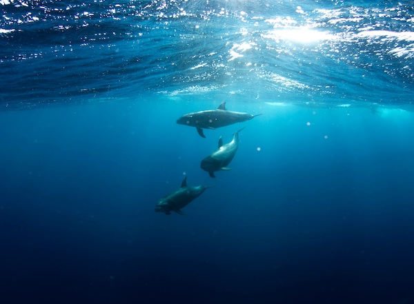
Even with images that you think might be hard, like this one that has multiple dolphins close together, and with their bodies mostly underwater, it does the right thing:
Like the previous AlexNet model we used for fine tuning, we can use GoogLeNet as well. Modifying the network is a bit trickier, since you have to redefine three fully connected layers instead of just one.
To fine tune GoogLeNet for our use case, we need to once again create a new Classification Model:
We rename all references to the three fully connected classification layers,
loss1/classifier, loss2/classifier, and loss3/classifier, and redefine
the number of categories (num_output: 2). Here are the changes we need to make
in order to rename the 3 classifier layers, as well as to change from 1000 to 2 categories:
@@ -917,10 +917,10 @@
   exclude { stage: "deploy" }
 }
 layer {
-  name: "loss1/classifier"
+  name: "loss1a/classifier"
   type: "InnerProduct"
   bottom: "loss1/fc"
-  top: "loss1/classifier"
+  top: "loss1a/classifier"
   param {
     lr_mult: 1
     decay_mult: 1
@@ -930,7 +930,7 @@
     decay_mult: 0
   }
   inner_product_param {
-    num_output: 1000
+    num_output: 2
     weight_filler {
       type: "xavier"
       std: 0.0009765625
@@ -945,7 +945,7 @@
 layer {
   name: "loss1/loss"
   type: "SoftmaxWithLoss"
-  bottom: "loss1/classifier"
+  bottom: "loss1a/classifier"
   bottom: "label"
   top: "loss1/loss"
   loss_weight: 0.3
@@ -954,7 +954,7 @@
 layer {
   name: "loss1/top-1"
   type: "Accuracy"
-  bottom: "loss1/classifier"
+  bottom: "loss1a/classifier"
   bottom: "label"
   top: "loss1/accuracy"
   include { stage: "val" }
@@ -962,7 +962,7 @@
 layer {
   name: "loss1/top-5"
   type: "Accuracy"
-  bottom: "loss1/classifier"
+  bottom: "loss1a/classifier"
   bottom: "label"
   top: "loss1/accuracy-top5"
   include { stage: "val" }
@@ -1705,10 +1705,10 @@
   exclude { stage: "deploy" }
 }
 layer {
-  name: "loss2/classifier"
+  name: "loss2a/classifier"
   type: "InnerProduct"
   bottom: "loss2/fc"
-  top: "loss2/classifier"
+  top: "loss2a/classifier"
   param {
     lr_mult: 1
     decay_mult: 1
@@ -1718,7 +1718,7 @@
     decay_mult: 0
   }
   inner_product_param {
-    num_output: 1000
+    num_output: 2
     weight_filler {
       type: "xavier"
       std: 0.0009765625
@@ -1733,7 +1733,7 @@
 layer {
   name: "loss2/loss"
   type: "SoftmaxWithLoss"
-  bottom: "loss2/classifier"
+  bottom: "loss2a/classifier"
   bottom: "label"
   top: "loss2/loss"
   loss_weight: 0.3
@@ -1742,7 +1742,7 @@
 layer {
   name: "loss2/top-1"
   type: "Accuracy"
-  bottom: "loss2/classifier"
+  bottom: "loss2a/classifier"
   bottom: "label"
   top: "loss2/accuracy"
   include { stage: "val" }
@@ -1750,7 +1750,7 @@
 layer {
   name: "loss2/top-5"
   type: "Accuracy"
-  bottom: "loss2/classifier"
+  bottom: "loss2a/classifier"
   bottom: "label"
   top: "loss2/accuracy-top5"
   include { stage: "val" }
@@ -2435,10 +2435,10 @@
   }
 }
 layer {
-  name: "loss3/classifier"
+  name: "loss3a/classifier"
   type: "InnerProduct"
   bottom: "pool5/7x7_s1"
-  top: "loss3/classifier"
+  top: "loss3a/classifier"
   param {
     lr_mult: 1
     decay_mult: 1
@@ -2448,7 +2448,7 @@
     decay_mult: 0
   }
   inner_product_param {
-    num_output: 1000
+    num_output: 2
     weight_filler {
       type: "xavier"
     }
@@ -2461,7 +2461,7 @@
 layer {
   name: "loss3/loss"
   type: "SoftmaxWithLoss"
-  bottom: "loss3/classifier"
+  bottom: "loss3a/classifier"
   bottom: "label"
   top: "loss"
   loss_weight: 1
@@ -2470,7 +2470,7 @@
 layer {
   name: "loss3/top-1"
   type: "Accuracy"
-  bottom: "loss3/classifier"
+  bottom: "loss3a/classifier"
   bottom: "label"
   top: "accuracy"
   include { stage: "val" }
@@ -2478,7 +2478,7 @@
 layer {
   name: "loss3/top-5"
   type: "Accuracy"
-  bottom: "loss3/classifier"
+  bottom: "loss3a/classifier"
   bottom: "label"
   top: "accuracy-top5"
   include { stage: "val" }
@@ -2489,7 +2489,7 @@
 layer {
   name: "softmax"
   type: "Softmax"
-  bottom: "loss3/classifier"
+  bottom: "loss3a/classifier"
   top: "softmax"
   include { stage: "deploy" }
 }
I’ve put the complete file in src/googlenet-customized.prototxt.
Q: "What about changes to the prototext definitions of these networks? We changed the fully connected layer name(s), and the number of categories. What else could, or should be changed, and in what circumstances?"
Great question, and it's something I'm wondering, too. For example, I know that we can "fix" certain layers so the weights don't change. Doing other things involves understanding how the layers work, which is beyond this guide, and also beyond its author at present!
Like we did with fine tuning AlexNet, we also reduce the learning rate by
10% from 0.01 to 0.001.
Q: "What other changes would make sense when fine tuning these networks? What about different numbers of epochs, batch sizes, solver types (Adam, AdaDelta, AdaGrad, etc), learning rates, policies (Exponential Decay, Inverse Decay, Sigmoid Decay, etc), step sizes, and gamma values?"
Great question, and one that I wonder about as well. I only have a vague understanding of these and it’s likely that there are improvements we can make if you know how to alter these values when training. This is something that needs better documentation.
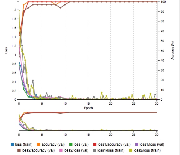
Because GoogLeNet has a more complicated architecture than AlexNet, fine tuning it requires more time. On my laptop, it takes 10 minutes to retrain GoogLeNet with our dataset, achieving 100% accuracy and a loss of 0.0070:
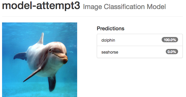
Just as we saw with the fine tuned version of AlexNet, our modified GoogLeNet performs amazing well--the best so far:
##Using our Model
With our network trained and tested, it’s time to download and use it. Each of the models
we trained in DIGITS has a Download Model button, as well as a way to select different
snapshots within our training run (e.g., Epoch #30):

Clicking Download Model downloads a tar.gz archive containing the following files:
deploy.prototxt
mean.binaryproto
solver.prototxt
info.json
original.prototxt
labels.txt
snapshot_iter_90.caffemodel
train_val.prototxt
There’s a nice description in the Caffe documentation about how to use the model we just built. It says:
A network is defined by its design (.prototxt), and its weights (.caffemodel). As a network is being trained, the current state of that network's weights are stored in a .caffemodel. With both of these we can move from the train/test phase into the production phase.
In its current state, the design of the network is not designed for deployment. Before we can release our network as a product, we often need to alter it in a few ways:
- Remove the data layer that was used for training, as for in the case of classification we are no longer providing labels for our data.
- Remove any layer that is dependent upon data labels.
- Set the network up to accept data.
- Have the network output the result.
DIGITS has already done the work for us, separating out the different versions of our prototxt files.
The files we’ll care about when using this network are:
deploy.prototxt- the definition of our network, ready for accepting image input datamean.binaryproto- our model will need us to subtract the image mean from each image that it processes, and this is the mean image.labels.txt- a list of our labels (dolphin,seahorse) in case we want to print them vs. just the category numbersnapshot_iter_90.caffemodel- these are the trained weights for our network
We can use these files in a number of ways to classify new images. For example, in our
CAFFE_ROOT we can use build/examples/cpp_classification/classification.bin to classify one image:
$ cd $CAFFE_ROOT/build/examples/cpp_classification
$ ./classification.bin deploy.prototxt snapshot_iter_90.caffemodel mean.binaryproto labels.txt dolphin1.jpg
This will spit out a bunch of debug text, followed by the predictions for each of our two categories:
0.9997 - “dolphin”
0.0003 - “seahorse”
You can read the complete C++ source for this in the Caffe examples.
For a classification version that uses the Python interface, DIGITS includes a nice example.
Finally, there's a fairly well documented Python walkthrough in the Caffe examples.
I wish I had more and better documented code examples, APIs, premade modules, etc to show you here. To be honest, most of the code examples I’ve found are terse, and poorly documented--Caffe’s documentation is spotty, and assumes a lot. It seems to me like there’s an opportunity for someone to build higher-level tools on top of the Caffe interfaces for beginners. It would be great if there were more simple modules in high-level languages that I could point you at that “did the right thing” with our model; someone could/should take this on, and make using Caffe models as easy as DIGITS makes training them. I’d love to have something I could use in node.js, for example. Ideally one shouldn’t be required to know so much about the internals of the model or Caffe. I haven’t used it yet, but DeepDetect looks interesting on this front, and there are likely many other tools I don’t know about.
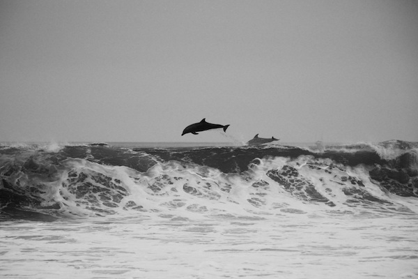
At the beginning we said that our goal was to write a program that used a neural network to correctly classify all of the images in data/untrained-samples. These are images of dolphins and seahorses that were never used in the training or validation data:
Let's look at how each of our three attempts did with this challenge:
| Image | Dolphin | Seahorse | Result |
|---|---|---|---|
| dolphin1.jpg | 71.11% | 28.89% | 😑 |
| dolphin2.jpg | 99.2% | 0.8% | 😎 |
| dolphin3.jpg | 63.3% | 36.7% | 😕 |
| seahorse1.jpg | 95.04% | 4.96% | 😞 |
| seahorse2.jpg | 56.64% | 43.36 | 😕 |
| seahorse3.jpg | 7.06% | 92.94% | 😁 |
| Image | Dolphin | Seahorse | Result |
|---|---|---|---|
| dolphin1.jpg | 99.1% | 0.09% | 😎 |
| dolphin2.jpg | 99.5% | 0.05% | 😎 |
| dolphin3.jpg | 91.48% | 8.52% | 😁 |
| seahorse1.jpg | 0% | 100% | 😎 |
| seahorse2.jpg | 0% | 100% | 😎 |
| seahorse3.jpg | 0% | 100% | 😎 |
| Image | Dolphin | Seahorse | Result |
|---|---|---|---|
| dolphin1.jpg | 99.86% | 0.14% | 😎 |
| dolphin2.jpg | 100% | 0% | 😎 |
| dolphin3.jpg | 100% | 0% | 😎 |
| seahorse1.jpg | 0.5% | 99.5% | 😎 |
| seahorse2.jpg | 0% | 100% | 😎 |
| seahorse3.jpg | 0.02% | 99.98% | 😎 |
##Conclusion
It’s amazing how well our model works, and what’s possible by fine tuning a pretrained network. Obviously our dolphin vs. seahorse example is contrived, and the dataset overly limited--we really do want more and better data if we want our network to be robust. But since our goal was to examine the tools and workflows of neural networks, it’s turned out to be an ideal case, especially since it didn’t require expensive equipment or massive amounts of time.
Above all I hope that this experience helps to remove the overwhelming fear of getting started. Deciding whether or not it’s worth investing time in learning the theories of machine learning and neural networks is easier when you’ve been able to see it work in a small way. Now that you’ve got a setup and a working approach, you can try doing other sorts of classifications. You might also look at the other types of things you can do with Caffe and DIGITS, for example, finding objects within an image, or doing segmentation.
Have fun with machine learning!
