Cascade Skills Assessment: dbt Data Engineer

This repository contains my submission for the Cascade Data Engineer skills assessment. The original assessment instructions can be found here. My dbt project is contained in the dbt/ directory. Instructions for running the dbt project can be found in dbt/README.md.

Model Lineage and Data Modeling

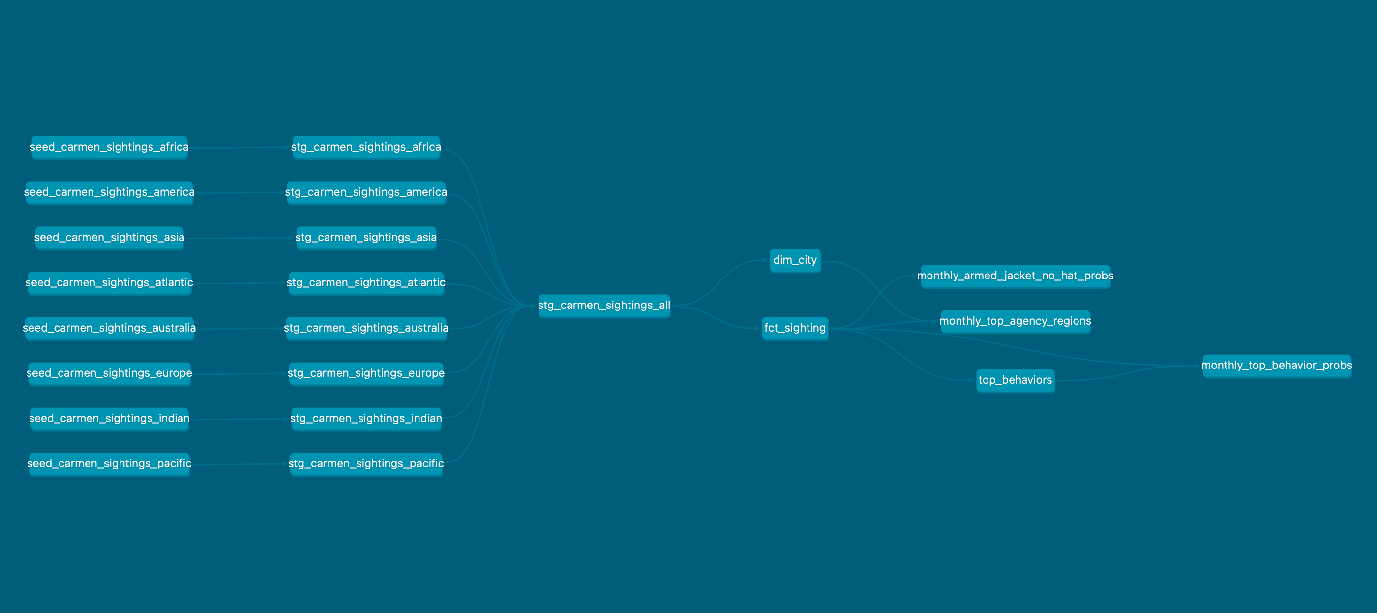
The image above displays the complete dag for the data models in this project. The dag is composed of several sequential segments:

1. The raw source data, consisting dbt seeds.
2. Staging models, materialized as views. These models either rename or concatenate source data.
3. Fact and dimension models, materialized as tables. These models form the core basis for downstream analytics.
4. Analytics models, materialized as views.

1. Source data

The source data is broken out into 8 seeds, each containing sightings for a different region. Different seeds may use different column names, but they all record data using the same format.

2. Staging

The staging models add uniformity to the seed models. Each seed has a corresponding staging view that applies a consistent column name mapping. In addition, the stg_carmen_sightings_all model concatenates all the upstream staging models so that all source sighting data can be easily queried at once.

3. Dimensional Models

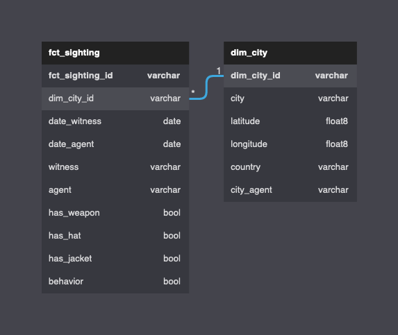
The "core" data models of this project consist of a fact and dimension table. They are both built off of the stg_carmen_sightings_all view.

• fct_sighting contains one record for each sighting.
• dim_city contains one record for each city where a sighting occurred.

When designing this schema, I assumed all the columns in dim_city remain constant per city (including city_agent). This assumption is valid for all the data used in this project, and can be verified via the uniqueness constraints placed on the dim_city_id column. However, if this assumption were not to hold for future data, then the current schema would need to be adjusted (e.g. dim_city could be modeled as a slowly changing dimension, or additional data models could be introduced)

4. Relationship Diagram

The image below depict the relationship between fct_sighting and dim_city. Note that there is a many-to-one relationship between fct_sighting and dim_city. When writing queries, city data can be added to sighting records by joining fct_sighting and dim_city on the dim_city_id column. This column has been indexed to facilitate fast joins using the indexes model config key, although this index would be much more useful if the the tables contained more rows.

Analytical Views

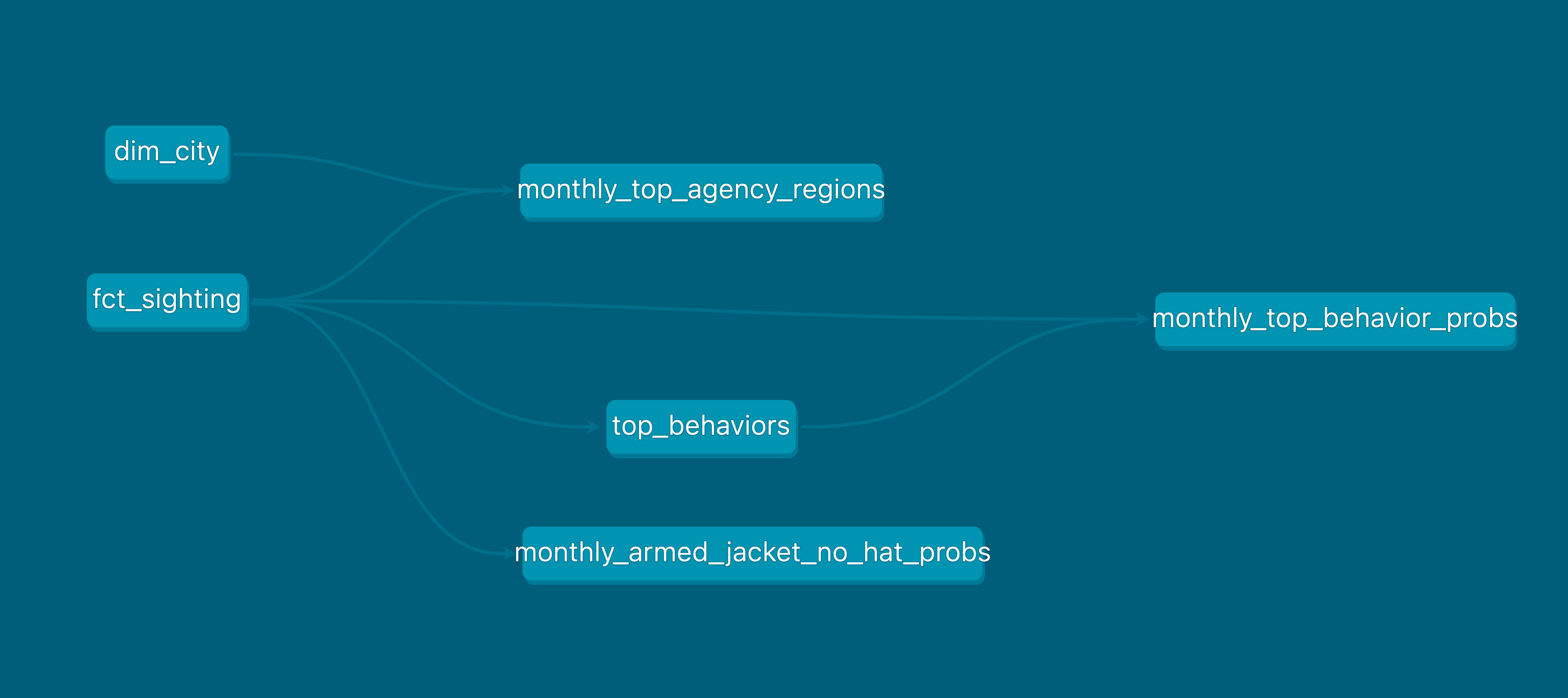
Analytical views exist downstream of the dimensional models. The dag below depicts the data lineage, starting from the dimensional models. Each analytical view contains at most two upstream dependencies, which are typically fct_sighting or dim_city. The monthly_top_behavior view references references top_behavior view because it makes use of its findings.

Analytical views that depict quantities by month use a custom month format defined in the format_date_to_month macro. This combines the month number (for sortability) with the month name (for readability).

The analytical view functions often use a similar approach of grouping sightings by month and use staple SQL functions by applying row_number over a window for ranking and using sum and count to compute proportions.

Analytics Questions

The analytical questions are answered below. Each answer makes use of one of the analytical view models depicted above.

a. For each month, which agency region is Carmen Sandiego most likely to be found?

The data from the monthly_top_agency_regions shows that Carmen Sandiego is most likely to be found in Kolkata or New York, depending on the month:

month_sighted	city_agent	times_observed	round
january	Kolkata	98	0.085
february	New York	86	0.082
march	New York	89	0.078
april	New York	91	0.081
may	Kolkata	94	0.080
june	Kolkata	83	0.073
july	New York	94	0.082
august	Kolkata	88	0.077
september	New York	71	0.064
october	New York	69	0.060
november	New York	93	0.084
december	Kolkata	94	0.082

b. Also for each month, what is the probability that Ms. Sandiego is armed AND wearing a jacket, but NOT a hat? What general observations about Ms. Sandiego can you make from this?

The data table, created from the monthly_armed_jacket_no_hat_probs view, is displayed below. The probabilities of the combined behaviors is very low for each month, hovering roughly between 3% and 5%. The month with the lowest probability is November, at 2.4%. The month with the highest probability is June, at 4.7%.

month_sighted	round
january	0.038
february	0.033
march	0.046
april	0.032
may	0.035
june	0.047
july	0.038
august	0.044
september	0.043
october	0.043
november	0.024
december	0.045

c. What are the three most occurring behaviors of Ms. Sandiego?

Carmen Sandiego's most occurring behaviors are happy, complaining, and out-of-control. The top_behaviors view was used to generate the table below.

behavior	times_observed
happy	635
complaining	636
out-of-control	637

d. For each month, what is the probability Ms. Sandiego exhibits one of her three most occurring behaviors?

The probability of a sighting containing the behavior happy, complaining, or out-of-control hovers between 12% and 15% each month. This is lowest in October, at 12.1%, and highest in May, at 15.3%.

month_sighted	round
january	0.139
february	0.138
march	0.149
april	0.138
may	0.153
june	0.138
july	0.139
august	0.138
september	0.150
october	0.121
november	0.144
december	0.138