Importando pyband: arduino Copy code import pyband Usando pyband para gerar sequências de banda aleatórias: perl Copy code seq = pyband.gen_seq(length=10) print(seq) Usando pyband para gerar uma sequência de banda com base em uma sequência de entrada: makefile Copy code input_seq = "ATCG" band_seq = pyband.band(input_seq) print(band_seq) Importando stockpyl: arduino Copy code import stockpyl Usando stockpyl para obter o preço de fechamento de uma ação em um determinado dia: bash Copy code ticker = "AAPL" date = "2022-01-01" closing_price = stockpyl.get_closing_price(ticker, date) print(closing_price) Usando stockpyl para obter o preço de fechamento de uma ação em um determinado intervalo de datas: makefile Copy code ticker = "AAPL" start_date = "2022-01-01" end_date = "2022-01-31" closing_prices = stockpyl.get_closing_prices(ticker, start_date, end_date) print(closing_prices) Importando mind-discord: arduino Copy code import mind_discord Autenticando com a API do Discord: makefile Copy code client = mind_discord.DiscordClient(token="YOUR_DISCORD_TOKEN") Obtendo informações sobre um servidor do Discord: makefile Copy code server_id = "1234567890" server_info = client.get_server_info(server_id) print(server_info) Obtendo informações sobre um canal do Discord: makefile Copy code channel_id = "1234567890" channel_info = client.get_channel_info(channel_id) print(channel_info) Enviando uma mensagem para um canal do Discord: makefile Copy code channel_id = "1234567890" message = "Hello, world!" client.send_message(channel_id, message) Obtendo a lista de membros de um servidor do Discord: makefile Copy code server_id = "1234567890" member_list = client.get_member_list(server_id) print(member_list) Obtendo a lista de canais de um servidor do Discord: makefile Copy code server_id = "1234567890" channel_list = client.get_channel_list(server_id) print(channel_list) Criando um novo canal em um servidor do Discord: makefile Copy code server_id = "1234567890" channel_name = "new-channel" client.create_channel(server_id, channel_name) network error
pyband and pydos are two python scripts that analyse the VASP calculation
results (e.g. OUTCAR and PROCAR) and convert the results to images. It offers a
fast and effective way to preview the calcuated results. The image plotting
utilizes matplotlib package.
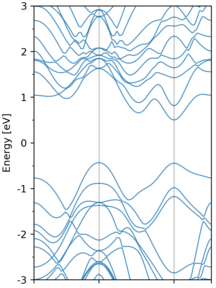
When no argument is given, pyband reads in OUTCAR (optionally KPOINTS)
and find the band information within. It then plots the resulting band structure
and save it as band.png.
$ pyband
The default output image name can be changed by adding -o YourImageName.suffix to the above command line. Note that the image format is
automatically recognized by the script, which can be any format that is
supported by matplotlib. The size of the image can also be speified by -s width height command line arguments.
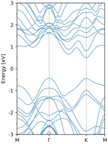
The labels of the high-symmetry K-points, which are not shown in the figure, can
be designate by -k flag.
$ pyband -k mgkm
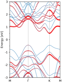
In some cases, if you are interested in finding out the characters of each KS
states, e.g. the contribution of some atom to each KS state, the flag --occ atoms comes to help.
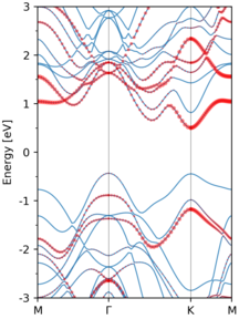
$ pyband --occ '1 3 4'
or
$ pyband --occ '1-4'
or combination
$ pyband --occ '1-4 5-6 7'
Note the the index 0 is a special one, it is used select all the atoms
$ pyband --occ 0
where 1 3 4 are the atom index starting from 1 to #atoms in the above image.
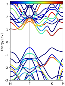
The size of red dots in the figure indicates the weight of the specified atoms
to the KS states. This can also be represented using a colormap:
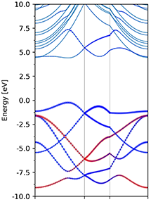
$ pyband --occ '1 3 4' --occL
The spd-projected weight can also be specefied:
$ pyband --occ '1 3 4' --spd '4 5 6 7 8'
or
$ pyband --occ '1 3 4' --spd 'd'
or in combination
$ pyband --occ '1 3 4' --spd 's p d 9-12'
where in the arguments of --spd:
s orbital: 0
py, pz, px orbital: 1 2 3
dxy, dyz, dz2, dxz, dx2 orbital: 4 5 6 7 8
More command line arguments can be found by pyband -h.
For Mac users, iterm2 combined with imgcat can be used to show inline images. Just modify the last line from:
call(['feh', '-xdF', opts.bandimage])
to
call(['~/.iterm2/imgcat', opts.bandimage])
more example:
pyband --occ '3 4' --spd '1' --occMc 'red' --occ '3-4' --spd '2-3' --occMc 'blue'
pyband command produces plotable data with a GNUPLOT compatiable format. Files are named "pyband.dat" for spinless or SOC calculations and "pyband_up(do).dat" for spinfull calculations. Plot the bandsturcture by:
$ gnuplot -presist -e 'plot "pyband.dat" u 1:($2-3.0913) w l'
This script is used to plot partial density of states (pDOS) from VASP PROCAR
files.
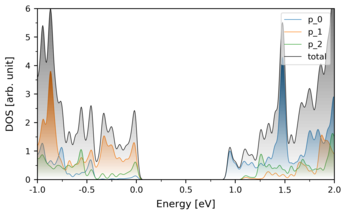
pydos -p '1 3 4' -p '2 7 8' -p '5 6 9' -z 0.65 -x -1 2 -y 0 6
where -p specifies the atom indexes, -x and -y determines the x and y
limits of the plot, -z is followed by the energy reference of the plot.
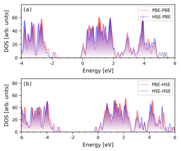
This script can plot PDOS from multiple VASP PROCARs in multiple axes, example usages:
#!/bin/bash

npdos -nr 2 -f 4.8 4.0 \
    -o g1.png \
    -nxminor 4 \
    -i pbe/scf/PROCAR         -a 0 -p 0 -pv n -tlab 'PBE-PBE' -tlw 0.5 -tlc r \
    -i scf-pbe_opt-hse/PROCAR -a 0 -p 0 -pv n -tlab 'HSE-PBE' -tlw 0.5 -tlc b \
    -i scf-hse_opt-pbe/PROCAR -a 1 -p 0 -pv n -tlab 'PBE-HSE' -tlw 0.5 -tlc r \
    -i hse/scf/PROCAR         -a 1 -p 0 -pv n -tlab 'HSE-HSE' -tlw 0.5 -tlc b \
    -x -4 6 -x -6 6 \
    -z 3.3129 -z 3.3726 -z 3.5583 -z 3.6332 \
    -panelloc 0.01 0.95 \
    -q
The resulting figure:
This script utilize ASE to make
supercells. The coordinates of the atoms in the resulting supercell is
rearranged in the increasing order in the z-axis. It can also rearrange the
elements in POSCAR in the required order. Moreover, vacuum can be added in the
desired direction if specified. Examples usage:
xcell.py -i POSCAR -s 2 2 1 -n Ti O C H -vacuum 15 -ivacuum z -o new.vasp
In the above example, we are makeing a 2x2x1 supercell based on the cell given
by POSCAR. The elements in the supercell are arranged in "Ti O C H" order. In
addition, we add a vacuum of 15 Angstrom in the z-axis. The resulting supercell
is stored in the file new.vasp.
This script also make use of ASE to adsorb molecules onto the slab surface.
Examples usage:
molAdd.py -m H2O -i POSCAR -a 36 --height 2.0 -rotx 60 -v 15.0
where we add a H2O molecule above the atom with index 36 (which is the 37th
atom) by a height of 2.0 Angstrom. In addition, we rotate the molecule around
x-axis by 60 degrees and add 15.0 Angstrom of vacuum to the slab. The list of
available molecules is those from ase.collection.g2 database.
