The Deep Learning Book - Goodfellow, I., Bengio, Y., and Courville, A. (2016)
This content is part of a series following the chapter 2 on linear algebra from the Deep Learning Book by Goodfellow, I., Bengio, Y., and Courville, A. (2016). It aims to provide intuitions/drawings/python code on mathematical theories and is constructed as my understanding of these concepts.
I'd like to introduce a series of blog posts and their corresponding Python Notebooks gathering notes on the Deep Learning Book from Ian Goodfellow, Yoshua Bengio, and Aaron Courville (2016). The aim of these notebooks is to help beginners/advanced beginners to grasp linear algebra concepts underlying deep learning and machine learning. Acquiring these skills can boost your ability to understand and apply various data science algorithms. In my opinion, it is one of the bedrock of machine learning, deep learning and data science.
These notes cover the chapter 2 on Linear Algebra. I liked this chapter because it gives a sense of what is most used in the domain of machine learning and deep learning. It is thus a great syllabus for anyone who wants to dive in deep learning and acquire the concepts of linear algebra useful to better understand deep learning algorithms.
You can find all the articles here.
The goal of this series is to provide content for beginners who want to understand enough linear algebra to be confortable with machine learning and deep learning. However, I think that the chapter on linear algebra from the Deep Learning book is a bit tough for beginners. So I decided to produce code, examples and drawings on each part of this chapter in order to add steps that may not be obvious for beginners. I also think that you can convey as much information and knowledge through examples as through general definitions. The illustrations are a way to see the big picture of an idea. Finally, I think that coding is a great tool to experiment with these abstract mathematical notions. Along with pen and paper, it adds a layer of what you can try to push your understanding through new horizons.
Graphical representation is also very helpful to understand linear algebra. I tried to bind the concepts with plots (and code to produce it). The type of representation I liked most by doing this series is the fact that you can see any matrix as linear transformation of the space. In several chapters we will extend this idea and see how it can be useful to understand eigendecomposition, Singular Value Decomposition (SVD) or the Principal Components Analysis (PCA).
In addition, I noticed that creating and reading examples is really helpful to understand the theory. It is why I built Python notebooks. The goal is two folds:
-
To provide a starting point to use Python/Numpy to apply linear algebra concepts. And since the final goal is to use linear algebra concepts for data science, it seems natural to continuously go between theory and code. All you will need is a working Python installation with major mathematical librairies like Numpy/Scipy/Matplotlib.
-
Give a more concrete vision of the underlying concepts. I found hugely useful to play and experiment with these notebooks in order to build my understanding of somewhat complicated theoretical concepts or notations. I hope that reading them will be as useful.
The syllabus follows exactly the Deep Learning Book so you can find more details if you can't understand one specific point while you are reading it. Here is a short description of the content:
-
Scalars, Vectors, Matrices and Tensors
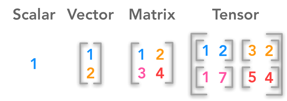
Difference between a scalar, a vector, a matrix and a tensor
Light introduction to vectors, matrices, transpose and basic operations (addition of vectors of matrices). Introduces also Numpy functions and finally a word on broadcasting.
-
Multiplying Matrices and Vectors
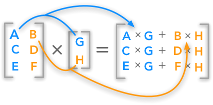
The dot product explained
This chapter is mainly on the dot product (vector and/or matrix multiplication). We will also see some of its properties. Then, we will see how to synthesize a system of linear equations using matrix notation. This is a major process for the following chapters.
-
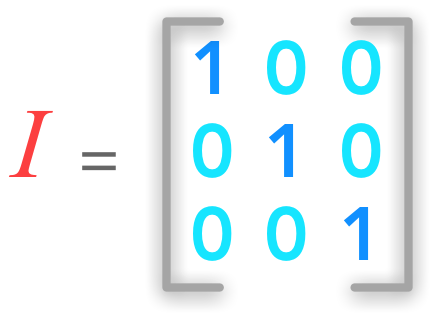
An identity matrix
We will see two important matrices: the identity matrix and the inverse matrix. We will see why they are important in linear algebra and how to use them with Numpy. Finally, we will see an example on how to solve a system of linear equations with the inverse matrix.
-

A system of equations has no solution, 1 solution or an infinite number of solutions
In this chapter we will continue to study systems of linear equations. We will see that such systems can't have more than one solution and less than an infinite number of solutions. We will see the intuition, the graphical representation and the proof behind this statement. Then we will go back to the matrix form of the system and consider what Gilbert Strang calls the row figure (we are looking at the rows, that is to say multiple equations) and the column figure (looking at the columns, that is to say the linear combination of the coefficients). We will also see what is linear combination. Finally, we will see examples of overdetermined and underdetermined systems of equations.
-

Shape of a squared L2 norm in 3 dimensions
The norm of a vector is a function that takes a vector in input and outputs a positive value. It can be thought of as the length of the vector. It is for example used to evaluate the distance between the prediction of a model and the actual value. We will see different kinds of norms (
$L^0$ ,$L^1$ ,$L^2$ ...) with examples. -
Special Kinds of Matrices and Vectors
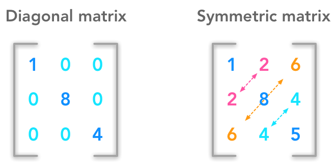
A diagonal (left) and a symmetric matrix (right)
We have seen in 2.3 some special matrices that are very interesting. We will see other types of vectors and matrices in this chapter. It is not a big chapter but it is important to understand the next ones.
-
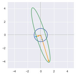
We will see some major concepts of linear algebra in this chapter. We will start by getting some ideas on eigenvectors and eigenvalues. We will see that a matrix can be seen as a linear transformation and that applying a matrix on its eigenvectors gives new vectors with same direction. Then we will see how to express quadratic equations in a matrix form. We will see that the eigendecomposition of the matrix corresponding to the quadratic equation can be used to find its minimum and maximum. As a bonus, we will also see how to visualize linear transformation in Python!
-
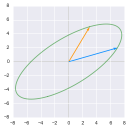
We will see another way to decompose matrices: the Singular Value Decomposition or SVD. Since the beginning of this series I emphasized the fact that you can see matrices as linear transformation in space. With the SVD, you decompose a matrix in three other matrices. We will see that we look at these new matrices as sub-transformation of the space. Instead of doing the transformation in one movement, we decompose it in three movements. As a bonus, we will apply the SVD to image processing. We will see the effect of SVD on an example image of Lucy the goose. So keep on reading!
-
The Moore-Penrose Pseudoinverse
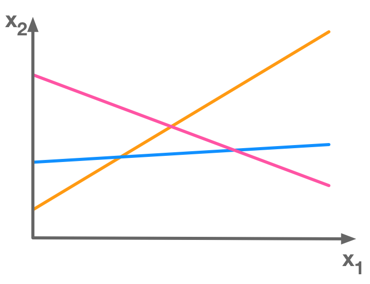
We saw that not all matrices have an inverse. It is unfortunate because the inverse is used to solve system of equations. In some cases, a system of equations has no solution, and thus the inverse doesn’t exist. However it can be useful to find a value that is almost a solution (in terms of minimizing the error). This can be done with the pseudoinverse! We will see for instance how we can find the best-fit line of a set of data points with the pseudoinverse.
-
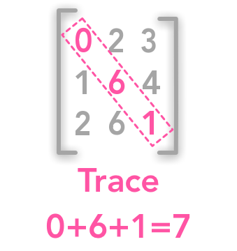
The trace of matrix
We will see what is the Trace of a matrix. It will be needed for the last chapter on the Principal Component Analysis (PCA).
-

Link between the determinant of a matrix and the transformation associated with it
This chapter is about the determinant of a matrix. This special number can tell us a lot of things about our matrix!
-
Example: Principal Components Analysis
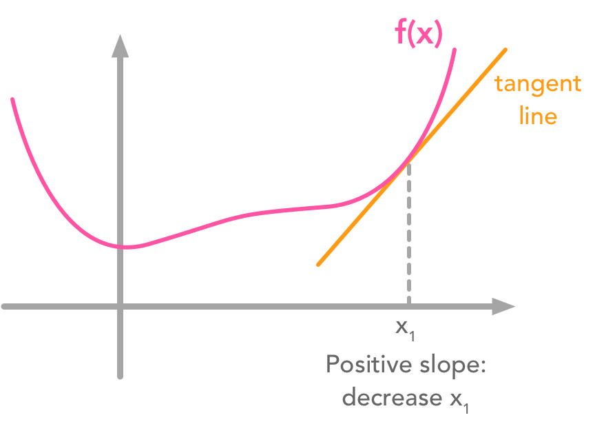 **Gradient descent**
This is the last chapter of this series on linear algebra! It is about Principal Components Analysis (PCA). We will use some knowledge that we acquired along the preceding chapters to understand this important data analysis tool!
This content is aimed at beginners but it would be nice to have at least some experience with mathematics.
I hope that you will find something interesting in this series. I tried to be as accurate as I could. If you find errors/misunderstandings/typos… Please report it! You can send me emails or open issues and pull request in the notebooks Github.
Goodfellow, I., Bengio, Y., & Courville, A. (2016). Deep learning. MIT press.
