Project: Pick & Place for Product (Object) sorting by Robotic Arm (Willow Garage PR2): Amazon Robotics Chanage, 2017

This project focuses on 3D perception using a PR2 robot simulation utilizing an RGB-D camera. The goal of perception is to convert sensor input into a point cloud image where specific objects can be identified and isolated.

The three main parts of perception include filtering the point cloud, clustering relevant objects and recognizing objects (Exercise 3), and then, the last part, using all perception steps in ROS environment for perception pick and place by a PR2 Robot.

3D Perception Pipeline:

1. Pipeline for filtering and RANSAC plane fitting implemented.

In this step, my pipeline is as follows:

Image -> Voxel Grid Downsampling -> Passthrough over Axis -> Outlier Filter -> RANSAC PLANE Filter -> Done

For each of these sections, I'll list the details:

1. Convert the point cloud which is passed in as a ROS message to PCL format.

2. Filter out the camera noise with the PCL statistical outlier filter. The adjustable parameters are the number k of neighbouring pixels to average over and the outlier threshold thr = mean_distance + x * std_dev. I used the RViz output image to tune these parameters judging by the visual output. For the PR2 simulation, I found that a mean k value of 20 and a standard deviation threshold of 0.1 provided the optimal outlier filtering and removing as much noise as possible without deleting content.

3. Downsample the image with a PCL voxel grid filter to reduce processing time and memory consumption. The adjustable parameter is the leaf size which is the side length of the voxel cube to average over. A leaf size of 0.01 seemed a good compromise between gain in computation speed and resolution loss.

4. A passthrough filter to define the region of interest and to isolate the table and objects. This filter clips the volume to the specified range. My region of interest is within the range 0.76 < z < 1.1.

5. RANSAC plane segmentation in order to separate the table from the objects on it. A maximum threshold of 0.01 worked well to fit the geometric plane model. The cloud is then segmented in two parts the table (inliers) and the objects of interest (outliers). The segments are published to ROS as /pcl_table and /pcl_objects. From this point onwards the objects segment of the point cloud is used for further processing. Here is the objects cloud after RANSAC segmentation for the objects and extraced the table and outliers for world 3 environment with 8 different objects:

2. Pipeline including clustering for segmentation implemented.

In order to detect individual objects, the point cloud needs to be clustered.

Following the lectures I applied Euclidean clustering. The parameters that worked best for me are a cluster tolerance of 0.05, a minimum cluster size of 100 and a maximum cluster size of 3000. The optimal values for Euclidean clustering depend on the leaf size defined above, since the voxel grid determines the point density in the image.

The search method is k-d tree, which is appropriate here since the objects are well separated the x and y directions (e.g seen when rotating the RViz view parallel to z-axis).

Performing a DBSCAN within the PR2 simulation required converting the XYZRGB point cloud to a XYZ point cloud, making a k-d tree (decreases the computation required), preparing the Euclidean clustering function, and extracting the clusters from the cloud. This process generates a list of points for each detected object.

By assigning random colors to the isolated objects within the scene, I was able to generate this cloud of objects:

The next part of the pipeline handles the actual object recognition using machine learning.

3. Features extracted and SVM trained. Object recognition implemented.

The object recognition code allows each object within the object cluster to be identified. In order to do this, the system first needs to train a model to learn what each object looks like. Once it has this model, the system will be able to make predictions as to which object it sees. To generate the training sets, I added the items from pick_list_3.yaml, which contains all object models, to the capture_features_project.py script:

    models = [\
       'biscuits',
       'soap',
       'soap2',
       'book',
       'glue',
       'sticky_notes',
       'snacks',
       'eraser']

For engineering the features I assumed (following the lectures) that an object is characterized by the following properties:

• the distribution of color channels,
• the distribution of surface normals.

Color histograms are used to measure how each object looks when captured as an image. Each object is positioned in random orientations to give the model a more complete understanding. For better feature extraction, the RGB image can be converted to HSV before being analyzed as a histogram. The number of bins used for the histogram changes how detailed each object is mapped, however too many bins will over-fit the object. The code for building the histograms can be found in features.py. The capture_features_project.py script saved the object features to a file named training_set_project.sav. It captured each object in 100 random orientations and 32 bins when creating the image histograms. The color histograms are in HSV space with range (0, 256) and the surface normal histograms have a range of (-1, 1).

Train SVM Model

A support vector machine (SVM) is used to train the model (specifically a SVC). The SVM loads the training set generated from the capture_features_pr2.py script, and prepares the raw data for classification. I found that a linear kernel using a C value of 0.1 builds a model with good accuracy.

I experimented with cross validation of the model and found that a 50 - 70 fold cross validation worked best. A leave one out cross validation strategy provided marginally better accuracy results, however, it required much longer to process. This model reached an accuracy score of 0.93 in cross-validation and later on successfully detected all objects in the test scenes 1, 2 and one missing object (glue) in test scene 3. The following figure shows the normalized confusion matrix produced by the train_svm.py script.

The trained model is then used in the pcl_callback routine to infer class labels from the given clusters. This means for each cluster in the list the features are calculated and then the classifier predicts the most probable object label. These labels are published to /object_markers and the detected objects of type DetectedObject() are published to /detected_objects. Then the pr2_mover routine is called in order to generate a ROS message for each detected object.

Pick and Place Setup

1. For all three tabletop setups (test*.world), perform object recognition, then read in respective pick list (pick_list_*.yaml). Next construct the messages that would comprise a valid PickPlace request output them to .yaml format.

Results

In the final configuration, the perception pipeline recognized all objects in all the test scenes. The screenshots below show clippings of the RViz window subscribed to the /pcl_objects publisher. The objects in the scene are labeled with the predicted label.

Scene 1

See the file output_1.yaml and the screenshot below.

Scene 2

See the file output_2.yaml and the screenshot below.

Scene 3

See the file output_3.yaml and the screenshot below.

Improvements

The performance of the pipeline depends on the perception parameters and the machine learning model. So the main improvements can be made in the following three categories.

• Parameter tuning. Adjust perception parameters to the camera hardware in use and the application. For example, adapt to changing region of interest and object distribution in the scene.
• Find a better feature engineering such as doing a grid search to find the parameters that optimize the accuracy score, and choosing a better the machine learning model to optimize the object recognition, for instance, change the Kernel type of the SVM (in this project the linear kernel performs better than RBF) or impelement more sophisticated deep learning techniques.

Project Setup

For this setup, catkin_ws is the name of active ROS Workspace, if your workspace name is different, change the commands accordingly If you do not have an active ROS workspace, you can create one by:

$ mkdir -p ~/catkin_ws/src
$ cd ~/catkin_ws/
$ catkin_make

Now that you have a workspace, clone or download this repo into the src directory of your workspace.

Note: If you have the Kinematics Pick and Place project in the same ROS Workspace as this project, please remove the 'gazebo_grasp_plugin' directory from the project directory otherwise ignore this note.

Now install missing dependencies using rosdep install:

$ cd ~/catkin_ws
$ rosdep install --from-paths src --ignore-src --rosdistro=kinetic -y

Build the project:

$ cd ~/catkin_ws
$ catkin_make

Add following to your .bashrc file

export GAZEBO_MODEL_PATH=~/catkin_ws/src/Amazon-Robotics-Challenge-with-PR2-Robot-Pick-and-Place-for-object-sorting/pr2_robot/models:$GAZEBO_MODEL_PATH

If you haven’t already, following line can be added to your .bashrc to auto-source all new terminals

source ~/catkin_ws/devel/setup.bash

To run the demo:

$ cd ~/catkin_ws/src/Amazon-Robotics-Challenge-with-PR2-Robot-Pick-and-Place-for-object-sorting/pr2_robot/scripts
$ chmod u+x pr2_safe_spawner.sh
$ ./pr2_safe_spawner.sh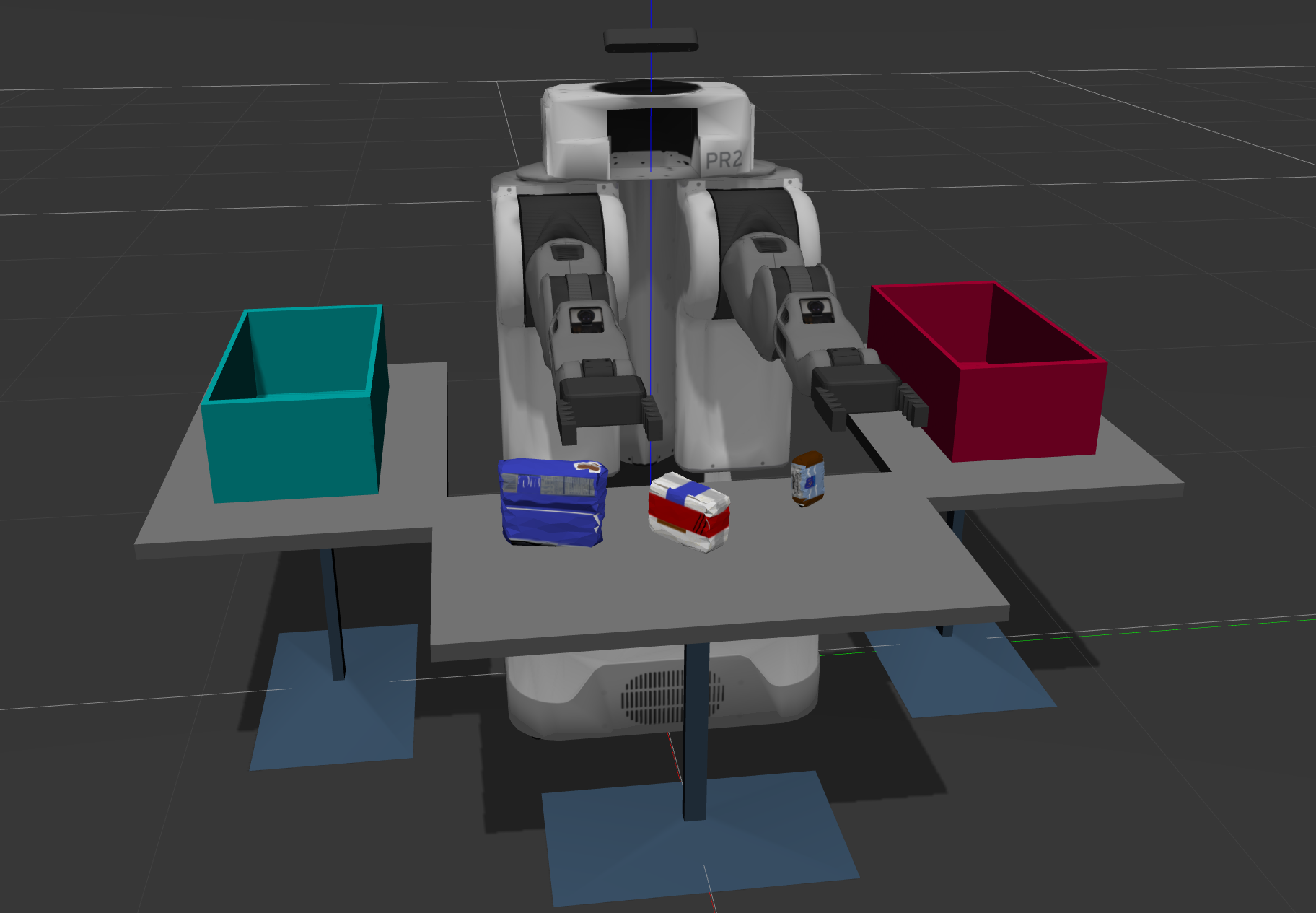

Once Gazebo is up and running, make sure you see following in the gazebo world:

• Robot

• Table arrangement

• Three target objects on the table

• Dropboxes on either sides of the robot

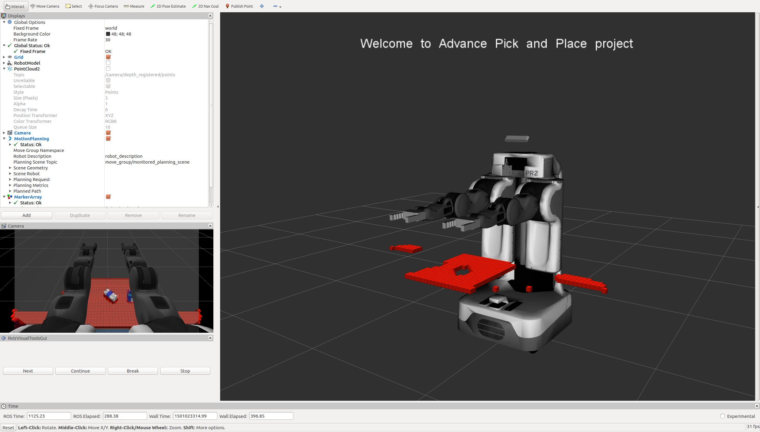
In your RViz window, you should see the robot and a partial collision map displayed:

Proceed through the demo by pressing the ‘Next’ button on the RViz window when a prompt appears in your active terminal

The demo ends when the robot has successfully picked and placed all objects into respective dropboxes (though sometimes the robot gets excited and throws objects across the room!)

Close all active terminal windows using ctrl+c before restarting the demo.

You can launch the project scenario like this:

$ roslaunch pr2_robot pick_place_project.launch