Lane and Vehicle Detection for Self-Driving Cars

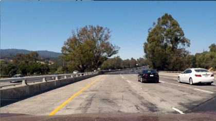
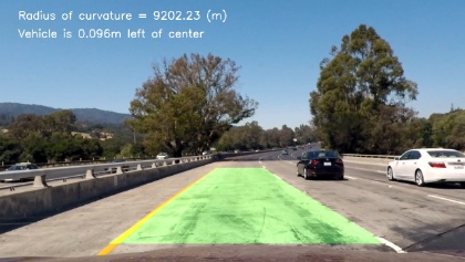
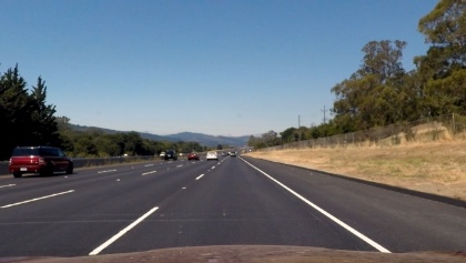
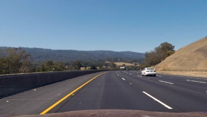
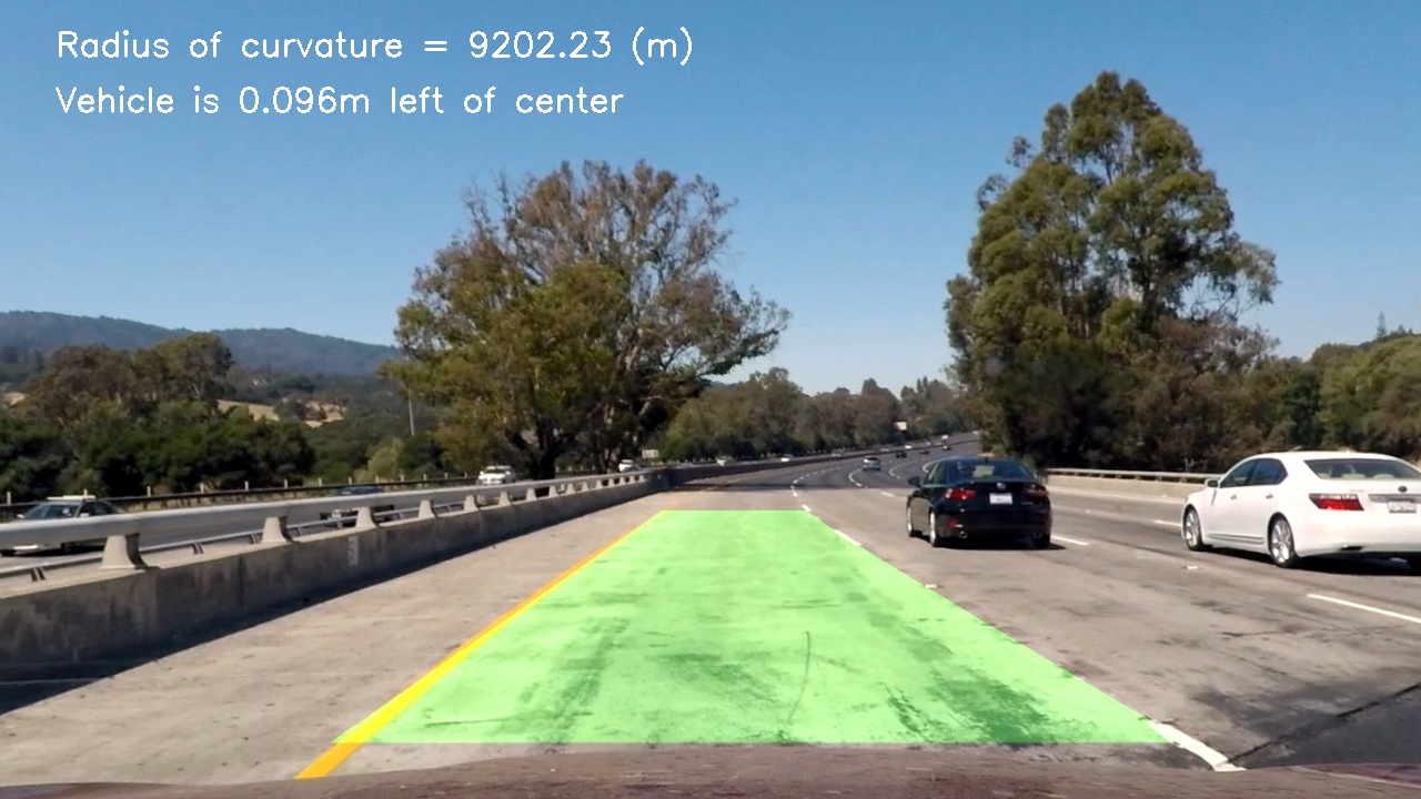
The goal of this project is to produce a robust pipeline for detecting lane lines and surrounding vehicles given an image from a front-facing monocular camera. The pipeline should output a visual display of the lane boundaries, numerical estimation of lane curvature, the vehicle's position within the lane, and bounding boxes drawn around nearby vehicles.

Lane Detection

Files and Usage

1. camera_cal.py
   • Contains code for calibrating the camera to undistort images.
   • python camera_cal.py will return the camera matrix and distortion coefficients and save them in a pickle file calibration_pickle.p.
2. thresholds.py
   • Contains code for applying color and gradient thresholds to an image to better detect lane lines.
3. lane_tracker.py
   • Contains code for identifying lane lines and highlighting the lane boundaries.
4. process_video.py
   • Contains code to generate a video with lane boundaries applied to an input video.
   • python process_video.py will save the output video as project_video_out.mp4 in the output_videos/ directory.
5. image_generator.py
   • Contains code to generate images with lane boundaries applied to the test images from a dashcam.
   • python image_generator.py will save the output images in the output_images folder.

Overview

The steps taken to complete this project are as follows:

• Compute the camera calibration matrix and distortion coefficients given a set of chessboard images.
• Apply a distortion correction to raw images.
• Use color transforms and gradients to create a thresholded binary image.
• Apply a perspective transform to rectify binary image ("birds-eye view").
• Detect lane pixels and fit to find the lane boundary.
• Determine the curvature of the lane and vehicle position with respect to center.
• Warp the detected lane boundaries back onto the original image.
• Output visual display of the lane boundaries, numerical estimation of lane curvature, and vehicle position.

Camera Calibration

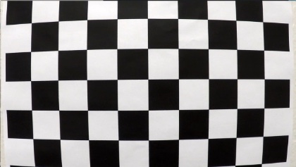
Cameras typically do not generate perfect images; some of the objects in the images can get stretched or skewed in various ways, especially near the edges. We can correct for this by performing a camera calibration. I started by preparing "object points", which will be the (x,y,z) coordinates of the chessboard corners in the world. The provided sample images of chessboards are fixed on the (x,y) plane at z=0, such that the object points are the same for each calibration image. Thus, objp is just a replicated array of coordinates, and objpoints will be appended with a copy of it every time all of the chessboard corners are successfully detected in a sample image. With each successful chessboard detection, imgpoints will be appended with the (x,y) pixel position of each of the corners. I then used the output objpoints and imgpoints to compute the camera calibration and distortion coefficients using the OpenCV calibrateCamera() function. The resulting camera matrix and distortion coefficients are then used to undistort images using the OpenCV undistort() function. Here an original image (left) and an undistorted image (right):

The code for camera calibration is contained in camera_cal.py and the sample images and outputs can be found in the camera_cal folder.

Distortion Correction

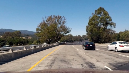
Using the camera matrix and distortion coefficients produced in the previous step, I undistort all incoming raw images using the OpenCV undistort() function. I use this function in my apply_lines() function which can be seen on line 38 of the lane_tracker.py file. Notice the difference in position of the white car between the raw image (left) and undistorted image (right):

Thresholded Binary Images

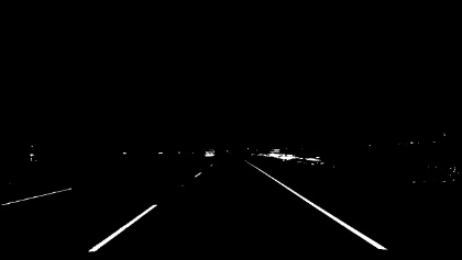
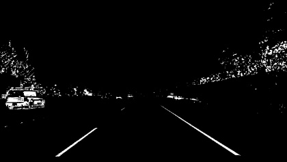
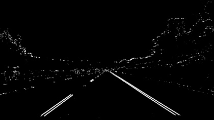
In order to accurately find the lane lines in an image, I applied a number of thresholding techniques to filter out potential noise (such as shadows, different color lanes, other cars, etc). I first applied a color threshold, where I save only the R (red) channel of the RGB image, and combine it with the S (saturation) channel of the image after converting it to HLS space. The reason I keep the red channel is because it does a good job of preserving the lanes in the image, but especially the yellow lane which other filters sometimes fail to detect. The binary image of the R channel (left) and the S channel (right) can be seen below:

Next, I apply thresholds on the gradients using the OpenCV Sobel() function. I apply a threshold on the magnitude of the gradient to filter out weak signals using the mag_thresh() function which can be found starting on line 6 of the thresholds.py file. I apply a threshold on the direction of the gradient in order to filter out horizonal lines, as the lane lines should be relatively vertical. You can find this dir_thresh() function starting on line 30 of the thresholds.py file. The binary image using the magnitude threshold (left) and directional threshold (right) can be seen below:

The binary images produced when combining both color thresholds (left) and both gradient thresholds (right):

I then combine the color and gradient thresholded binary images to produce the final binary image used in the pipeline for detecting the lane lines. You can see the original undistorted image (left) compared with the thresholded binary image (right) below:

The code for producing the thresholded binary images can be found in thresholds.py and some sample output images can be found in the output_images folder.

Perspective Transform

A perspective transform maps the points in a given image to a different, desired, image points with a new perspective. I use the OpenCV functions getPerspectiveTransform() and warpPerspective() to generate a bird's-eye view of a lane from above, which is useful for calculating the lane curvature. I chose the source points and destination points used to perform the transform following the example given in the course:

src = np.float32(
    [[(img_size[0] / 2) - 55, img_size[1] / 2 + 100],
    [((img_size[0] / 6) - 10), img_size[1]],
    [(img_size[0] * 5 / 6) + 60, img_size[1]],
    [(img_size[0] / 2 + 55), img_size[1] / 2 + 100]])
dst = np.float32(
    [[(img_size[0] / 4), 0],
    [(img_size[0] / 4), img_size[1]],
    [(img_size[0] * 3 / 4), img_size[1]],
    [(img_size[0] * 3 / 4), 0]])

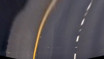
Using these points resulted in the following undistorted image (left) transformed to a bird's-eye perspective (right):

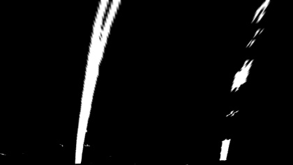
Below is the same applied to the thresholded binary image as described in the previous step:

The code for performing the perspective transform can be found on lines 54-70 of the lane_tracker.py file.

Detect Lane Pixels and Fit Lines

To find the pixels of the lane lines I take a histogram of the thresholded binary image by adding up the pixel values along each column in the lower half of the image using np.sum(img[img.shape[0]/2:,:], axis=0) as seen on line 85 of the lane_tracker.py file. Since pixels are either 0 or 1 in my binary image, the two most prominent peaks in the histogram will be good indicators of the x-position of the base of the lane lines. I then use that as a starting point for where to search for the lane lines, using a sliding window places around the line centers to find and follow the lines up to the top of the frame. A plot of such a histogram can be seen below:

After saving all of the pixel indices within the windows of interest, I use the numpy polyfit() function to fit a second order line to the pixels in the left and right lanes. To increase efficiency, after finding the lane lines I avoid doing an exhaustive search in subsequent frames by instead only searching within a margin around the previous found line positions. A plot of the search windows and the fitted lane lines are shown below:

The code to detect the lane pixels and fit the lines can be found on lines 80-146 of the lane_tracker.py file.

Determine Curvature of Lane and Vehicle Position

The radius of curvature of the lane at a particular point is defined as the radius of the approximating circle, which changes as we move along the curve. A good tutorial of the radius of curvature can be found here which describes the mathematical formula used to calculate it. In addition, I also needed to convert the radius from pixel values to real world space. I used the estimated figures given in the project lectures based on U.S. regulations that require a minimum lane width of 3.6 meters and dashed lane lines of 3 meters long each.

The code for calculating the radius of curvature can be found on lines 183-193 of the lane_tracker.py file.

To calculate the vehicle's position within the lane lines, I first assume that the car's dash cam is mounted at the center of the car. I then find the difference between the center of the image and the center of the two lane lines I've detected to determine the distance from the center of the lane (converted from pixels to meters).

The code for calculating the vehicle position can be found on lines 195-200 of the lane_tracker.py file.

Warp Detected Lane Boundaries onto Original Image

After detecting the lane lines, calculating the radius of curvature, and finding the vehicles position within the lane, I unwarp the image back to the original perspective using the OpenCV warpPerspective() function as before, but this time using the inverse matrix. This code can be found on line 174 of the lane_tracker.py file.

Visual Display of the Lane Boundaries, Curvature, and Vehicle Position

A link to my video result can be found here

Vehicle Detection