Wei Ding, Franz Baumdicker, Richard A Neher; panX: pan-genome analysis and exploration, Nucleic Acids Research, Volume 46, Issue 1, 9 January 2018, Pages e5, https://doi.org/10.1093/nar/gkx977
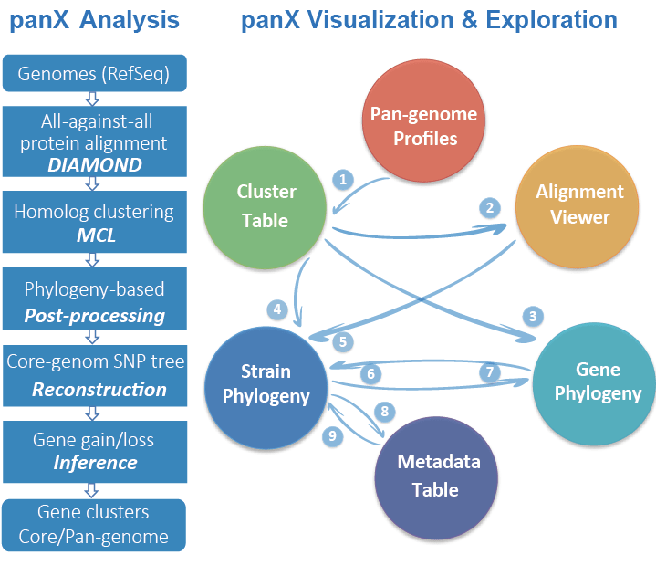
Overview: panX is a software package for microbial pan-genome analysis, visualization and exploration. The analysis pipeline is based on DIAMOND, MCL and phylogeny-aware post-processing. It takes a set of annotated bacterial strains as input (e.g. NCBI RefSeq records or user's own data in GenBank format). All genes from all strains are compared to each other via DIAMOND and then clustered into orthologous groups using MCL and adaptive phylogenetic post-processing, which split distantly related genes and paralogs if necessary. For each gene cluster, corresponding alignment and phylogeny are constructed. All core gene SNPs are then used to build strain/species phylogeny.
The results can be interactively explored using a powerful web-based visualization application (either hosted by web server or run locally on desktop). The web application integrates various interconnected components (pan-genome statistical charts, gene cluster table, alignment, comparative phylogenies, metadata table) and allows rapid search and filter of gene clusters by gene name, annotation, duplication, diversity, gene gain/loss events, etc. Strain-specific metadata are integrated into strain phylogeny such that genes related to adaptation, antibiotic resistance, virulence can be readily identified.
- Pipeline overview
- Quick start
- How to run
- Directory structure and analysis output
- Command line arguments
git clone https://github.com/neherlab/pan-genome-analysis.git
cd pan-genome-analysis
Install dependencies easily via Conda and then run the test:
sh run-TestSet.sh
The results can be explored using our interactive pan-genome-visualization application.
The required software and python packages can be readily installed using Conda.
wget https://repo.continuum.io/miniconda/Miniconda2-latest-Linux-x86_64.sh
bash Miniconda2-latest-Linux-x86_64.sh
export PATH=~/miniconda2/bin:$PATH
conda env create -f panX-environment.yml
source activate panX
To run the test set: sh run-TestSet.sh
In data/TestSet, you will find a small set of four Mycoplasma genitalium genomes that is used in this tutorial. Your own data should also reside in such a folder within data/ -- we will refer to this folder as run directory below. The name of the run directory is used as a species name in down-stream analysis.
All steps can be run in order by omitting the -st option, whereas using -st 5 6 will specify the analysis steps. If running only specific steps such as -st 5 6, steps before 5 should already be finished.
-t sets the number of CPU cores.
./panX.py -fn data/TestSet -sl TestSet -t 32 > TestSet.log 2> TestSet.err
This calls panX.py to run each step using scripts located in folder ./scripts/
./panX.py [-h] -fn folder_name -sl species_name
                   [-st steps [steps ...]] [-rt raxml_max_time]
                   [-t threads] [-bp blast_file_path]

Mandatory parameters: -fn folder_name / -sl species_name
NOTICE: species_name e.g.: S_aureus
Example: ./panX.py -fn ./data/TestSet -sl TestSet -t 32 > TestSet.log 2> TestSet.err
The analysis generates clustering result
./data/YourSpecies/allclusters_final.tsv
and files required for visualizing the pan-genome using pan-genome-visualization.
./data
    YourSpecies               # folder specific to the your pan genome
      - input_GenBank              # INPUT: genomes in GenBank format
        - strain1.gbk
        - strain2.gbk
        ...
      - vis
        - geneCluster.json       # for clusters table: gene clusters and their summary statistics
        - strainMetainfo.json    # for metadata table: strain-associated metadata
        - metaConfiguration.js   # metadata configuration file (also accept valid customized file)
        - coreGenomeTree.json    # core genome SNP tree (json file)
        - strain_tree.nwk        # core genome SNP tree (newick file)

        - geneCluster/           # folder contain orthologous clusters
                                 # nucleotide and amino acid alignment in gzipped FASTA format
                                 # reduced alignment contains a consensus sequence and variable sites (identical sites shown as dots)
                                 # tree and presence/absence(gain/loss) pattern in json format
          - GC00000001_na_aln.fa.gz
          - GC00000001_aa_aln.fa.gz
          - GC00000001_na_aln_reduced.fa.gz
          - GC00000001_aa_aln_reduced.fa.gz
          - GC00000001_tree.json
          - GC00000001_patterns.json
In which step different files and directories are produced is described in more details in step-tutorials.md.
Soft core-gene:
-cg    core-genome threshold [e.g.: 0.7] percentage of strains used to decide whether a gene is core
E.g.: ./panX.py -cg 0.7 -fn ...
Large dataset (use divide-and-conquer(DC) strategy which scales approximately linearly with the number of genomes):
-dmdc  apply DC strategy to run DIAMOND on subsets and then combine the results
-dcs   subset size used in DC strategy [default:50]
E.g.: ./panX.py -dmdc -dcs 50 -fn ...
Calculate branch associations with metadata (e.g. drug concentration):
-iba  infer_branch_association
-mtf  ./data/yourSpecies/meta_config.tsv
E.g.: ./panX.py -iba -mtf ./data/yourSpecies/meta_config.tsv -fn ...
Example: meta_config.tsv
To bring the branch association into effect for the visualization, one needs to add the generated file to the visualization repository as described in Special feature: visualize branch association(BA) and presence/absence(PA) association.
