Workshop Description

There are two steps to this OSM data analysis workshop:

1. First, we use Amazon Athena to query pre-processed OSM historical data.
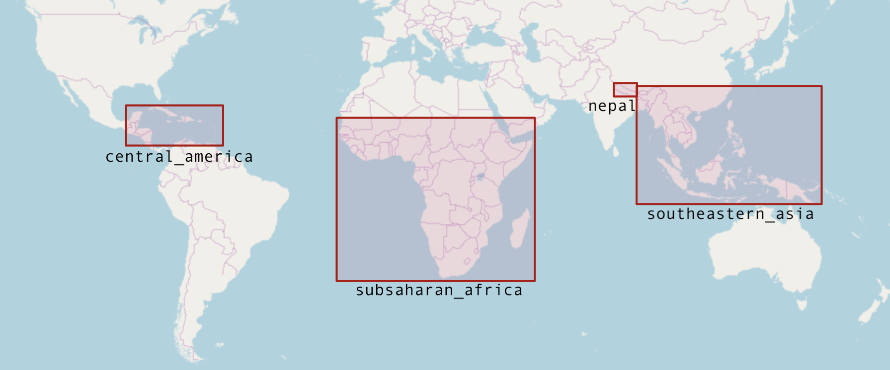
   • OSM historical editing data is currently available for the following areas. Database table names shown here:
   • All OSM changesets metadata is available
   • The pre-processed data exists as individual OSM objects with WKT geometries (not nodes/ways/relations)
   • The results of these queries are automatically saved to an Amazon S3 bucket.
2. Second, we use Jupyter Notebooks for an interactive analysis environment to download the query results from S3 and analyze/visualize.

Getting Started

Part 1: Amazon Athena

1. For this workshop we'll be sharing an AWS account. You can login here:

https://hot-aws-workshop.signin.aws.amazon.com/console

Use the following credentials where [NUMBER] is any number between 1 and 90: workshop-1, workshop-2, workshop-3, etc.

	username: workshop-[number]
	password: < see presentation slides> 

1. Go to the Amazon Athena console: https://us-east-2.console.aws.amazon.com/athena/home?region=us-east-2#query.

   Once logged in, double check that the region is set to us-east-2 (Ohio) because that is where the pre-processed OSM data lives. Not required, but if you'd like to change the workgroup, you can choose any of the other workshop groups by clicking on the Workgroup tab. This way you can save queries into a workgroup unique to you.

   

   Confirm that you are using the osm database. If there are no tables, see the Athena Setup instructions to load the tables.

2. Now you can begin querying the OSM data, see the Data section below for a more detailed description of what is attributes are available. Here are few queries to get you started and familiar with the interface.

   Copy the exact queries here and paste them into the query window.

   1. Count the number of users to ever work on a HOT task:

      SELECT count(DISTINCT(uid))
      FROM changesets
      WHERE lower(changesets.tags['comment']) LIKE '%hotosm%'

      It should return ~ 140,930. That's a lot of people. What about just this year?

      SELECT count(distinct(uid))
      FROM changesets
      WHERE lower(changesets.tags['comment']) LIKE '%hotosm%'
      	AND changesets.created_at > date '2019-01-01'

      This should return ~ 25,988. Wow, 25k mappers working on at least 1 hot task in 2019. What about users who have more than 1 HOT-related changeset?

      SELECT count(uid) FROM (
        SELECT uid, count(id) AS num_changesets
        FROM changesets
        WHERE lower(changesets.tags['comment']) LIKE '%hotosm%'
        GROUP BY uid
      ) WHERE num_changesets > 1

      ~ 121,860, implying only 20k users only made 1 changeset.

      These are simple results in which Athena is only returning single values. Let's dig into the data a bit more...

   2. Find all HOT-related changesets, grouped by user with basic per-user statistics.

       SELECT
           changesets.user,
           min(created_at) AS first_edit,
           max(created_at) AS last_edit,
           date_diff('day', min(created_at), max(created_at)) AS lifespan,
           sum(num_changes) AS total_edits
       FROM
           changesets
       WHERE
           changesets.tags['comment'] LIKE '%hotosm%' -- hotosm changesets only
       GROUP BY
           changesets.user
       ORDER BY lifespan DESC

      The results from this query will be a CSV with ~ 140k rows, one per mapper:

      

      At the upper-right, there is a link to download the results as a CSV file. To explore these results in more depth, we will load these CSV files into a Jupyter Notebook, as described next. This is done by copying and pasting this link. You can do this with a right-click:

      

Part 2: Logging into the Jupyter Notebooks

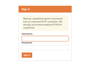
1. There is an instance of JupyterHub running on an Amazon EC2 machine located at workshop.yetilabs.science:8000 that will allow each workshop participant to run their own analysis environment.

   Similar to Athena, you can log in with the following credentials:

    username: workshop-[number]
   

   where [NUMBER] is any number between 1 and 90, examples: workshop-1, workshop-2, workshop-57, etc.

   Whatever password you enter when you first login will be the new password for this account. I suggest either leaving this blank or using hotsummit2019.

   

2. When you are successfully logged in and the notebook server is running, you should see a page that looks like this:

   

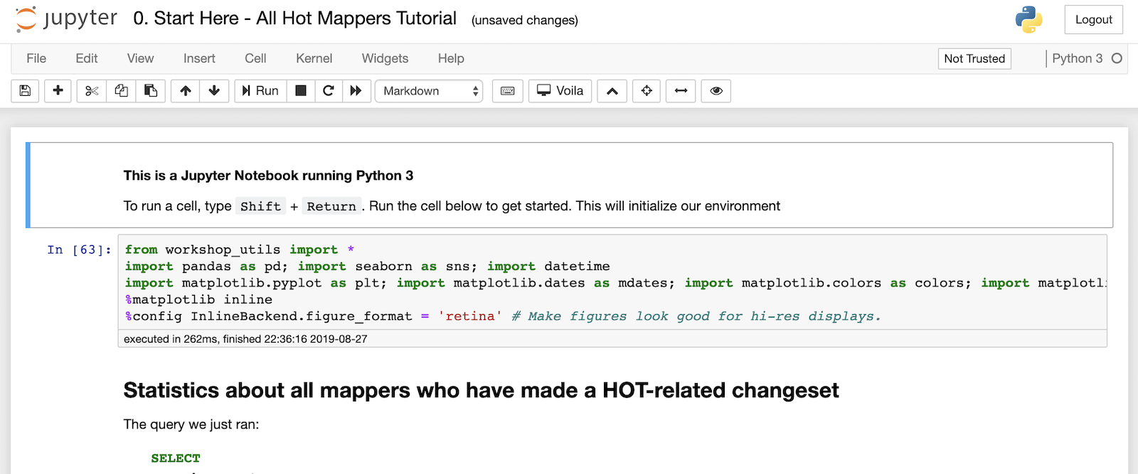
3. Click on the 0. Start Here - All Hot Mappers Tutorial.ipynb, when it starts, you should see this:

   

   Follow the directions in the notebook to load the CSV file from the previous query into the notebook and create a few charts.

Part 3: Other Notebooks

There are X numbered notebooks, (numbered for organization, not difficulty). They contain sample queries and the necessary code to analyze the results. Try them out and plug in your own spatial bounds to look at different areas.

Athena to Jupyter

Remember, when you run a new query in Athena, you need to copy the URL of the CSV file and paste that URL into the notebook to get the results from Athena to Jupyter

First, copy the URL from Athena:

Then paste it (with quotes) into the notebook, storing it as a variable like query:

query = "https://us-east-2.console.aws.amazon.com/athena/query/results/6cab4ea3-8431-4cd6-8f89-8881fa43c8b2/csv"

Then run run the load_dataframe_from_s3 function to get the query results into a Pandas Dataframe.

df = load_dataframe_from_s3(query)

Resources

1. For spatially bounded queries, this bounding box tool can quickly construct WKT bounding boxes. I recommend having this tool open in another tab for quick reference.

---

Data

Our dataset has gone through one step of pre-processing. Using the OSMesa utility, the raw node/way/relation elements have been converted into single OSM objects with WKT geometries. This conversion also accounts for minor versions, the unaccounted versions of ways and relations created by modifying the child object (like squaring a building or fixing a road).

Therefore the data looks slightly different from the original OSM data model, namely the following fields:

Attribute (Column)	Description
updated	When this version/minor version of the object was created
valid_until	When this particular version was altered, making this version of the object no longer the most recent
minor_version	How many times the geometry / child elements of the primary element has been modified
version	The version of this object that corresponds to the version of the OSM element
geom	The geometry of this version of the object (WKT)

---

Acknowledgements

This workshop is made possible by pre-processing the full-history editing record of OSM with OSM2ORC and OSMesa, and the help of Seth Fitzsimmons.

Jennings Anderson is a Postdoctoral Researcher at the University of Colorado Boulder. The preparation and design of this workshop is thereby supported by CU Boulder and the US National Science Foundation Grant IIS-1524806.

Amazon Web Services is providing computational resources, financial support, and planning / organizing the production of this workshop.