Generative diffusion-based downscaling for climate

Robbie A. Watt & Laura A. Mansfield https://arxiv.org/abs/2404.17752

This repo contains code to go alongside Watt & Mansfield (2024) preprint. In this preprint, we apply a diffusion based model and a Unet to a downscaling problem with climate data. The diffusion model is based on the implementation by T. Karras et al. (https://arxiv.org/abs/2206.00364) and the code is addapted from https://github.com/NVlabs/edm.

File structure

• src: contains code used to train model
• inference: contains inference and plotting scripts
• Model_chpt: contains model checkpoints
• download_ERA5: contains scripts for downloading ERA5 data and processing into netcdf files.

Usage

Download ERA5 data

The script download_ERA5/ERA5_download_my_dates_sfc.sh downloads the variables (temperature at 2m and zonal and meridional winds at 100 hPa) for all years of ERA5 up to 2022 and saves files into a directory named data/. You may need to edit data directories. Note that we subsample in time to reduce the size of the dataset (see file preprocessing_subsample.py). Data is concatenated into yearly samples and saved as samples_{year}.nc.

We also use variables that are constant in time for the land sea mask and the topography. These are currently stored in data/ERA5_const_sfc_variables.nc or can be manually downloaded from ERA5 Copernicus store ( https://cds.climate.copernicus.eu/cdsapp#!/dataset/reanalysis-era5-single-levels?tab=form) by checking geopotential (z) and land-sea mask (lsm) (found under Other) and saving these to netcdf.

Dependencies

python>=3.9, torch, tensorboard, xarray, netcdf4, cartopy, matplotlib, scipy, numpy

Training

To train either the diffusion or unet models from scratch, simply run the src/TrainDiffusion.py or src/TrainUnet.py script from the project root directory.

Inference

After training, the inference scripts can be run in the following order:

1. save_test_truth.py: this script simply processes the true test data to save it into one file for easier comparison to other variables
2. save_test_preds.py: this script runs through all test data and saves the output into one file. You need to run this for each model. modelname=UNet for the standard UNet, modelname=LinearInterpolation for linear interpolation of coarse resolution variables onto the high resolution grid (i.e., the inputs to the model) and modelname=Diffusion for the diffusion model. When running the Diffusion model, we generate many possible samples in a loop, each seeded with a different random number, currently we loop over rngs=range(0, 30).

After running the above scripts, you should have files saved as output/{modelname}/samples_2018-2023.nc (or for diffusion, these are saved as output/Diffusion/samples_{i}_2018-2023.nc where i indexes the different generated samples).

Plotting scripts:

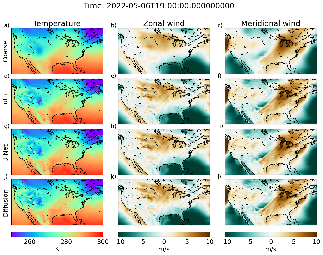
• plot_timestep_examples.py plots maps of methods for each timestep (used for Fig. 1).
• plot_error_metrics.py plots maps of error metrics across full test dataset (Fig. 2) and prints the mean across the domain.
• plot_spectrum.py plots the power spectrum for all methods (Fig. 3)

Citation

@misc{watt2024generative,
      title={Generative Diffusion-based Downscaling for Climate}, 
      author={Robbie A. Watt and Laura A. Mansfield},
      year={2024},
      eprint={2404.17752},
      archivePrefix={arXiv},
      primaryClass={physics.ao-ph}
}