| title | output | pagetitle |
|---|---|---|
README |
github_document |
README |
This package attempts to implement "parliament plots" - visual representations of the composition of legislatures that display seats colour-coded by party. The input is a data frame containing one row per party, with columns representing party name/label and number of seats, respectively.
This R package is a ggplot2 extension and is now on CRAN. Please install the stable version in R by running:
install.packages("ggparliament")To install the package from source:
devtools::install_github("robwhickman/ggparliament")Inspiration from this package comes from: parliamentdiagram, which is used on Wikipedia, parliament-svg, which is a javascript clone, and a discussion on StackOverflow, which provided some of the code for part for the "arc" representations used in this package.
If you have any issues, please note the problem and inform us!
ggparliament provides election data from the following countries.
election_data %>%
  distinct(year, country, house) %>%
  arrange(country, year)
## year country house
## 1 2010 Australia Representatives
## 2 2010 Australia Senate
## 3 2013 Australia Representatives
## 4 2013 Australia Senate
## 5 2016 Australia Representatives
## 6 2016 Australia Senate
## 7 2009 Chile Diputados
## 8 2009 Chile Senadores
## 9 2013 Chile Diputados
## 10 2013 Chile Senadores
## 11 2017 Chile Diputados
## 12 2017 Chile Senadores
## 13 1990 Germany Bundestag
## 14 1994 Germany Bundestag
## 15 1998 Germany Bundestag
## 16 2002 Germany Bundestag
## 17 2005 Germany Bundestag
## 18 2009 Germany Bundestag
## 19 2013 Germany Bundestag
## 20 2017 Germany Bundestag
## 21 2007 Russia Duma
## 22 2011 Russia Duma
## 23 2016 Russia Duma
## 24 2010 UK Commons
## 25 2015 UK Commons
## 26 2017 UK Commons
## 27 2012 USA Senate
## 28 2012 USA Representatives
## 29 2014 USA Senate
## 30 2014 USA Representatives
## 31 2016 USA Senate
## 32 2016 USA Representatives
We also provide the following vignettes for further explanation:
- Basic parliament plots
- Labelling parties
- Drawing the majority threshold line
- Highlighting parties in power
- Faceting legislatures
- Emphasizing certain seats
- Visualizaing overhang seats in MMP electoral systems
- Arranging seat order in ggparliament plots.
Quick ggparliament examples can be viewed below.
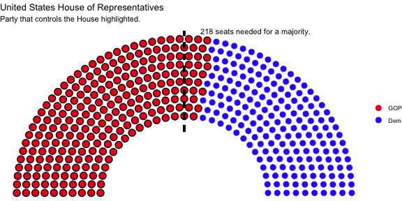
#filter the election data for the most recent US House of Representatives
us_house <- election_data %>%
  filter(country == "USA" &
    year == 2016 &
    house == "Representatives")

us_house <- parliament_data(election_data = us_house,
  type = "semicircle",
  parl_rows = 10,
  party_seats = us_house$seats)

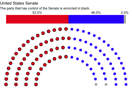
us_senate <- election_data %>%
  filter(country == "USA" &
    year == 2016 &
    house == "Senate")

us_senate <- parliament_data(
  election_data = us_senate,
  type = "semicircle",
  parl_rows = 4,
  party_seats = us_senate$seats)
representatives <- ggplot(us_house, aes(x, y, colour = party_short)) +
geom_parliament_seats() +
#highlight the party in control of the House with a black line
geom_highlight_government(government == 1) +
#draw majority threshold
draw_majoritythreshold(n = 218, label = TRUE, type = 'semicircle')+
#set theme_ggparliament
theme_ggparliament() +
#other aesthetics
labs(colour = NULL,
title = "United States House of Representatives",
subtitle = "Party that controls the House highlighted.") +
scale_colour_manual(values = us_house$colour,
limits = us_house$party_short)
representativessenate <- ggplot(us_senate, aes(x, y, colour = party_long)) +
geom_parliament_seats() +
geom_highlight_government(government == 1) +
# add bar showing proportion of seats by party in legislature
geom_parliament_bar(colour = colour, party = party_long) +
theme_ggparliament(legend = FALSE) +
labs(colour = NULL,
title = "United States Senate",
subtitle = "The party that has control of the Senate is encircled in black.") +
scale_colour_manual(values = us_senate$colour,
limits = us_senate$party_long)
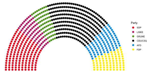
senate germany <- election_data %>%
filter(year == 2017 &
country == "Germany")
germany <- parliament_data(election_data = germany,
parl_rows = 10,
type = 'semicircle',
party_seats = germany$seats)
bundestag <- ggplot(germany, aes(x, y, colour = party_short)) +
geom_parliament_seats(size = 3) +
labs(colour="Party") +
theme_ggparliament(legend = TRUE) +
scale_colour_manual(values = germany$colour,
limits = germany$party_short)
bundestag#data preparation
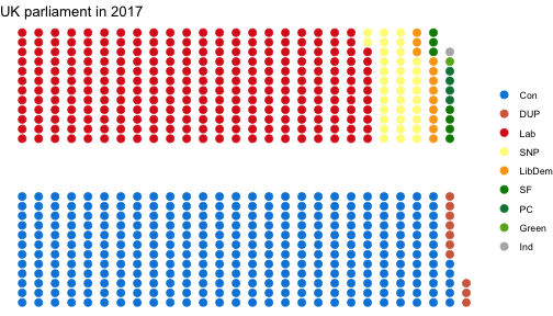
uk_17 <- election_data %>%
filter(country == "UK" &
year == "2017") %>%
parliament_data(election_data = .,
party_seats = .$seats,
parl_rows = 12,
type = "opposing_benches",
group = .$government)
commons <- ggplot(uk_17, aes(x, y, colour = party_short)) +
geom_parliament_seats(size = 3) +
theme_ggparliament() +
coord_flip() +
labs(colour = NULL,
title = "UK parliament in 2017") +
scale_colour_manual(values = uk_17$colour,
limits = uk_17$party_short)
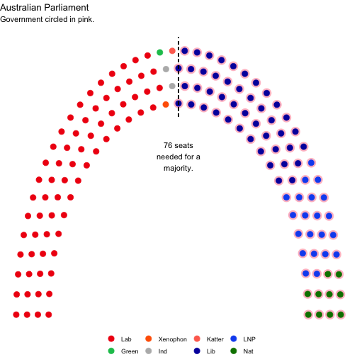
commonsaustralia <- election_data %>%
filter(country == "Australia" &
house == "Representatives" &
year == 2016) %>%
parliament_data(election_data = .,
party_seats = .$seats,
parl_rows = 4,
type = "horseshoe")au_rep <-ggplot(australia, aes(x, y, colour = party_short)) +
geom_parliament_seats(size = 3.5) +
geom_highlight_government(government == 1, colour = "pink", size = 4) +
draw_majoritythreshold(n = 76,
label = TRUE,
linesize = 0.5,
type = 'horseshoe') +
theme_ggparliament() +
theme(legend.position = 'bottom') +
labs(colour = NULL,
title = "Australian Parliament",
subtitle = "Government circled in pink.") +
scale_colour_manual(values = australia$colour,
limits = australia$party_short)
au_rep

