Open source project to bring data and ml to avalanche forecasting
Webpage is https://openavalancheproject.org Docs are located at https://scottcha.github.io/OpenAvalancheProject/
Directories are organized as follows:
-
Data
Contains files associated with data inputs, such as geojson definitions of avalanche regions. Training and label data are linked in the README there as they are too large to host in git.
-
DataPipelineNotebooks
The data prep code which is used to generate the OpenAvalanche pip package.
-
Environments
Conda environment yml files
-
Get Training Data
Files used to pull training data from various web sources
-
ML
Notebooks representing the current state of the art for danger prediction for this project
-
TestData
Sample test data supporting the automated tests
-
WebApp is the bulk of the operational code for the OAP website
- OpenAvalancheProjectWebApp Contains the code for the website
-
docs
Documentation generated with nbdev based on the notebooks in DataPipelineNotebooks
-
openavalancheproject.egg-info
Supporting pip package files generated with nbdev
-
openavalancheproject
Code generated with nbdev from DataPipelineNotebooks for the pip package
This aspect of the tutorial will cover how you can obtain new weather input data for a new date range or region. This part assumes you have avalanche forecast labels for the dates and region (OAP currently has historical forecast labels for three avalanche centers in the US from the 15-16 season through the 20-21 season and is working on expanding that).
Due to the large size of the input GFS data and the fact that its already hosted by NCAR, OAP isn't currently providing copies of this data. If you want to start a data processing pipeline from the original data you can start with this process here. If you aren't interested in the data processing steps and only in the ML steps you can download the labels here: https://github.com/scottcha/OpenAvalancheProject/blob/master/Data/CleanedForecastsNWAC_CAIC_UAC_CAC.V1.2013-2021.zip and a subset of training data here: [TODO: replace with current link] and skip to the fourth notebook 4.TimeseriesAi
The input data is derived from the .25 degree GFS model hosted by NCAR hosted at this site: https://rda.ucar.edu/datasets/ds084.1/
You'll need to create an account and once you are logged in you can visit the above link and then click on the Data Access tab. One note is that I've found that chromium based browsers don't work well on this site so I recommend you use Firefox for at least downloading the data.
Due to the size of the files we are downloading I only recommend downloading one season and for a regional subset at a time. In this example I'm going to download the data for Colorado.
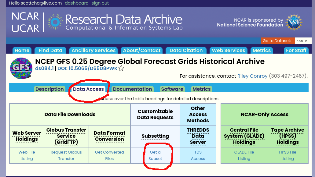 (note: the web ui has changed a bit since these screenshots were taken but the naivgation remains the same)
Click on the "Get a Subset" link.
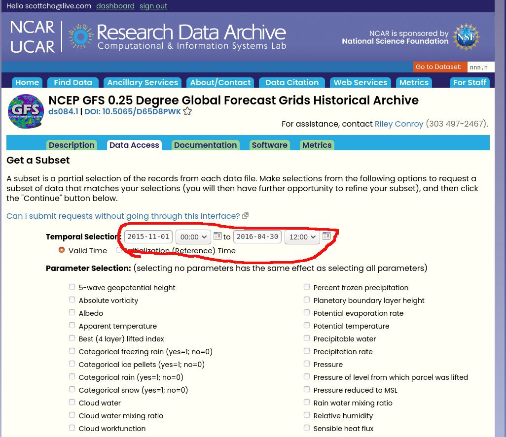
The next page allows us to select both the dates and parameters we are interested in. Currently we read all parameters so please check all parameters. For dates choose one winter season. In the below screenshot I've selected dates Nov 1, 2015 thorough April 30, 2016 for the 15-16 season. The models assume the season starts Nov 1 and ends April 30 (it wouldn't be too difficult to update the data pipeline for a southern hemisphere winter but its not something that has been done yet).
Click Continue and wait for it to validate your selections.
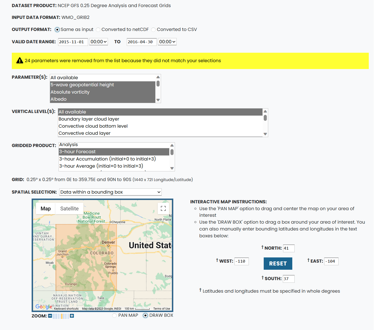
The next page allows you to further subset your data. There are a few important things here.
1. Verify that the dates are correct.
2. We want the output as grib (check "same as input")
3. Download all available vertical levels.
4. Select only the 3-24 hour forecasts and accumulation in the gridded products as currently OAP doesn't use more than this.
5. You can also then select the bounding box for the area you want to download in the "spatial selection". Once you have a bounding box you like write down the lat/lon values so its easier to input when we come back for other date ranges.
Once the selections are correct and you can eventually click through to submit your request. You should get a confirmation page of your selections and the system will start to retrieve your data. This usually takes a few hours and you will get an email when its ready for download. At this point if you want additional date/time ranges you can submit the requests and they will get queued and made avalable for download when they are ready. In this example the downloaded files were 1.1 GB.
Extract and decompress all the files until you have a per forecast grib file and ensure all the files have been moved in to a single directory (per season per location). If you are using Linux this stackoverflow post may help https://askubuntu.com/questions/146634/shell-script-to-move-all-files-from-subfolders-to-parent-folder.
Once you have all the files as grib files in a single directory for that date and location (i.e., 15-16/Colorado/) there are a couple final cleaning steps. Due to the download process sometimes some files earlier than 11/1 are included. You can just delete those files (the file date is 201510*)
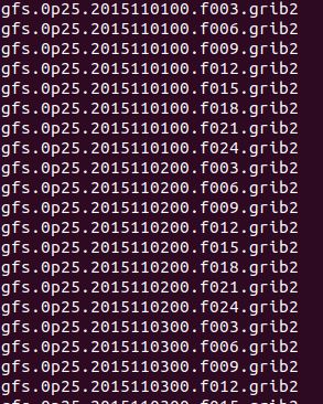
_Its worth a brief interlude in to understanding how these files are encoded. Here is a typical file name gfs.0p25.2015110100.f003.grib2. Lets break that down gfs: is the model we are using. 0p25 I beleive is the resolution at .25 degress but I haven't seen this documented. 2015110100 is the encoded date of the model runtime. You will see in your dataset that there are four models run per day: 00, 06, 12, 18. Currently we are only using the 00 model (the first of the day). The next component is .f003 which is the forecast for 3 hours from the model runtime. grib2 is the input file format. chamberlin455705 is the enocded download request.
Next delete all files which have a model run hour other than 00 (i.e., 06, 12, 18). Check that you have 1456 files at this point (8 files per day for 182 days, the data processing should be resiliant to the occasional missing file which does happen in these datasets). The total size of the input files at this point is ~270MB.
You will have to repeat the download process for the accumulation variables and place them in a parallel folder (see next; it is possible to add the accumulation variables to the single download but they need to be preprocessed differently so I prefer to keep them seperate).
The final step is to ensure the input data is in the correct folder structure. All data for this project will sit off a path you define as the base path. The GFS input data then needs to be in subfolders of that path delineated by season and state (or country). For example if our past path in this example is:
/media/scottcha/E1/Data/OAPMLData/
The place this data in
/media/scottcha/E1/Data/OAPMLData/1.RawWeatherData/15-16/Colorado/
or
/media/scottcha/E1/Data/OAPMLData/1.RawWeatherData/15-16/ColoradoAccumulationGrib/
[for the accumulation files]
Notes:
- There is an option to covert the file to NetCDF in the NCAR/UCAR UI. Don't use this as it will result in a .nc file which isn't in the same format as the one we are going to use.
Now that we have the input file set we can start to go through the initial data pipeline steps to transform and filter the data. Today this is done in a series of Jupyter notebooks. This format makes it easy to incrementally process and check the outputs while the project is in a development phase (once we have a model which seems to have a resonable output these steps will be encoded in a set of python modules and implemented as a processing pipeline).
Assuming you have Anaconda and Jupyter installed first change directory to the Environments directory at the root level of the repo. This contains two conda envrionment definitions, one for the processing steps, oap_ml_datapipeline.yml, and one for the deep learning step, oap_tsai.yml.
conda env create -f oap_datapipeline.yml
Once the environment has been created you can activate it with
conda activate oap_datapipeline
There is one step we need to take before going through the notebooks and that is converting the grib2 files to NetCDF. We do this for a couple of reasons but primarily that using this tool efficiently collapses the vertical dimensions (called level) in to the variable definitions so we can more easily get it to the ML format we need. The utility to do this is called wgrib2 and should have been installed in the oap_ml_datapipeline environment.
- While most of the data processing steps work equally well in Windows or Linux I've found the wgrib2 is much easier to install on a Linux environment so I tend to use Linux for at least the following step.
Using a terminal prompt change directory to the folder where you downloaded and unpacked the weather model files.
/media/scottcha/E1/Data/OAPMLData/1.RawWeatherData/15-16/Colorado/
In that directory you can execute this command to iterate through all the files and tranform them:
for i in *.grib2; do wgrib2 $i -netcdf $i.nc; done
There are ways of improving the efficiency by doing this in parallel so feel free to improve on this.
To start a new notebook launch jupyter
jupyter notebook
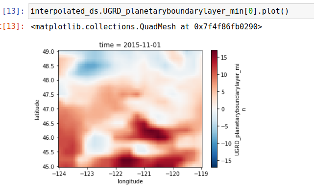
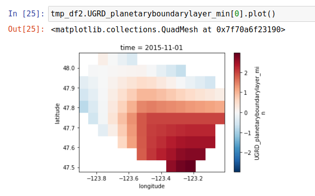
Completing these next few steps bascially takes the raw input weather data and leaves us with data slightly transformed but filtered to only the coordinates in the avalanche regions for that location. For example here is what a regional view of one of the parameters (U component of wind vector) looks like when both interpolated 4x and viewed across the entire Washington region:
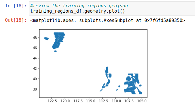
We've used this geojson definition of the avalanche regions to subset that view in to much smaller views focused on the avalanche forecast regions. Here are all the US regions.
And then this is what it looks like when filtered to only the Olympics avalanche region (the small one in the top left of the US regions):
Training labels can be downloaded here: https://github.com/scottcha/OpenAvalancheProject/blob/master/Data/CleanedForecastsNWAC_CAIC_UAC_CAC.V1.2013-2021.zip
1.RawWeatherData/
    gfs/
        <season>/
            /<state or country>/
2.GFSFiltered(x)Interpolation/
3.GFSFiltered(x)InterpolationZarr/
4.MLData
#test_ignore
season = '15-16'
state = 'Colorado'

interpolate = 1 #interpolation factor: whether we can to augment the data through lat/lon interpolation; 1 no interpolation, 4 is 4x interpolation

data_root = '/media/scottcha/E1/Data/OAPMLData/'

n_jobs = 24 #number of parallel processes to run
This code block will iterate through each season and region and produce the files for the next stage of te data pipeline.
for s in seasons:
    print("On season: " + s)
    pgfs = ParseGFS(s, state, data_root, resample_length='3H')
results = pgfs.resample_local(jobs=n_jobs)The next step in our data transformation pipeline is to transform the NetCDF files to Zarr files which are indexed in such a way to make access to specific dates and lat/lon pairs as efficient as possible. This process can be run entirely end to end once you are sure the parameters are set correctly. It does take about 2 hours for one season for all regions in Colorado on my workstation (12 core 3900X with data on Gen3 NVME drive) using all cores. The imporant item about this notebook is that we are essentially indexing the data to be accessed efficiently when we create our ML datasets.
#test_ignore
ctz = ConvertToZarr(seasons, regions, data_root)
#test_ignore
ctz.convert_local()This step needs to be run once to create a dataset to be used in a subsequent ML step. The way to think about these methods is that we use the set of valid labels + the valid lat/lon pairs as an index in to the data. Its important to understand the regions are geographically large and usually cover many lat/lon pairs in our gridded dataset while the labels apply to an entire region (multiple lat/lon pairs). For example the WA Cascades East, Central region coveres 24 lat/lon pairs so if on Jan 1 there was a label we wanted to predict our dataset would have 24 lat/lon pairs in that region associated with that label. There are pros and cons for this approach.
Pros:
- Reasonable data augmentation approach
- Aligns with how we utltimatly want to provide predictions--more granular, not restricted to established regions
Cons:
- Could be contributing to overfitting
- The data becomes very large
That being said the methods will calculate this index for every label/lat/lon point and then we'll split this in to train and test sets. Its important to ensure that the train test split is done in time (i.e., I usually use 15-16 through 18-19 as the training set and then 19-20 as the test set) as if you don't there will be data leakage.
Once the train test split is done on the labels there is a process to build up the dataset. This is still a slow process even when doing it in parallel and agains the indexed Zarr data. I've spent a lot of time trying various ways of optimizing this but I'm sure this could use more work. The primary method internal method for doign this is called get_xr_batch and takes several parameters:
- labels: list of the train or test set labels
- lookback_days: the number of previous days to include in the dataset. For example if the label is for Jan 1, then a lookback_days of 14 will also include the previous 14 days. I've been typically using 180 days as lookback (if a lookback extends prior to Nov 1 then we just fill in NaN as the data is likly irrelevant) but its possible that a lower value might give better results.
- batch_size: the size of the batch you want returned
- y_column: the label you want to use
- label_values: the possible values of the label from y_column. We include this as the method can implement oversampling to adjust for the imbalanced data.
- oversample: dict which indicates which labels should be oversampled.
- random_state: random variable initilizer
- n_jobs: number of processes to use
In the tutorial the notebook produced one train batche of 1,000 rows and one test batch of 500 rows and then concats them in a single memapped file.
#test_ignore
pml = PrepML(data_root, interpolate,  date_start='2015-11-01', date_end='2020-04-30', date_train_test_cutoff='2019-11-01')
#test_ignore
pml.regions = {
'Washington': ['Mt Hood', 'Olympics', 'Snoqualmie Pass', 'Stevens Pass',
'WA Cascades East, Central', 'WA Cascades East, North', 'WA Cascades East, South',
'WA Cascades West, Central', 'WA Cascades West, Mt Baker', 'WA Cascades West, South'
]}#test_ignore
%time train_labels, test_labels = pml.prep_labels()Mt Hood
Olympics
Snoqualmie Pass
Stevens Pass
WA Cascades East, Central
WA Cascades East, North
WA Cascades East, South
WA Cascades West, Central
WA Cascades West, Mt Baker
WA Cascades West, South
CPU times: user 19.6 s, sys: 531 ms, total: 20.2 s
Wall time: 20.4 s
#test_ignore
train_labels = train_labels[train_labels['UnifiedRegion'].isin(['Mt Hood',
                                                              'Olympics',
                                                              'Snoqualmie Pass',
                                                              'Stevens Pass',
                                                              'WA Cascades East, Central',
                                                              'WA Cascades East, North',
                                                              'WA Cascades East, South',
                                                              'WA Cascades West, Central',
                                                              'WA Cascades West, Mt Baker',
                                                              'WA Cascades West, South'])]
#test_ignore
test_labels = test_labels[test_labels['UnifiedRegion'].isin(['Mt Hood',
'Olympics',
'Snoqualmie Pass',
'Stevens Pass',
'WA Cascades East, Central',
'WA Cascades East, North',
'WA Cascades East, South',
'WA Cascades West, Central',
'WA Cascades West, Mt Baker',
'WA Cascades West, South'])]#test_ignore
train_labels.head().dataframe tbody tr th {
vertical-align: top;
}
.dataframe thead th {
text-align: right;
}
| UnifiedRegion | latitude | longitude | UnifiedRegionleft | Cornices_Likelihood | Cornices_MaximumSize | Cornices_MinimumSize | Cornices_OctagonAboveTreelineEast | Cornices_OctagonAboveTreelineNorth | Cornices_OctagonAboveTreelineNorthEast | ... | image_types | image_urls | rose_url | BottomLineSummary | Day1WarningText | Day2WarningText | parsed_date | season | Day1DangerAboveTreelineValue | Day1DangerAboveTreelineWithTrend | |
|---|---|---|---|---|---|---|---|---|---|---|---|---|---|---|---|---|---|---|---|---|---|
| 0 | Mt Hood | 45.25 | -121.75 | Mt Hood | no-data | no-data | no-data | no-data | no-data | no-data | ... | no-data | no-data | no-data | no-data | no-data | no-data | 2015-12-05 | 15-16 | 1.0 | Moderate_Initial |
| 1 | Mt Hood | 45.25 | -121.75 | Mt Hood | no-data | no-data | no-data | no-data | no-data | no-data | ... | no-data | no-data | no-data | no-data | no-data | no-data | 2015-12-06 | 15-16 | 1.0 | Moderate_Flat |
| 2 | Mt Hood | 45.25 | -121.75 | Mt Hood | no-data | no-data | no-data | no-data | no-data | no-data | ... | no-data | no-data | no-data | no-data | no-data | no-data | 2015-12-07 | 15-16 | 2.0 | Considerable_Rising |
| 3 | Mt Hood | 45.25 | -121.75 | Mt Hood | no-data | no-data | no-data | no-data | no-data | no-data | ... | no-data | no-data | no-data | no-data | no-data | no-data | 2015-12-08 | 15-16 | 2.0 | Considerable_Flat |
| 4 | Mt Hood | 45.25 | -121.75 | Mt Hood | no-data | no-data | no-data | no-data | no-data | no-data | ... | no-data | no-data | no-data | no-data | no-data | no-data | 2015-12-09 | 15-16 | 1.0 | Moderate_Falling |
5 rows × 302 columns
Note the class imbalance and the test set not having all classes. This isn't a good set for ML (one should use the entire 2015-2020 dataset but you need to ensure you have all the data from those dates available)
#test_ignore
train_labels['Day1DangerAboveTreeline'].value_counts()
Moderate 27982
Considerable 25588
High 5715
Low 2289
no-data 1272
Extreme 59
Name: Day1DangerAboveTreeline, dtype: int64
#test_ignore
test_labels['Day1DangerAboveTreeline'].value_counts()
Series([], Name: Day1DangerAboveTreeline, dtype: int64)
This will generate local files sampling from the datasets (parameters can specify exactly the amount of data to store) in the ML folder which can be used for the next ML process
Modifying the parameters so you don't run out of memory is important as its designed to append to the on disk files so as to stay within memory contraits: num_train_rows_per_file maxes out at around 50000 on my 48gb local machine. If you want more data than then then use num_train_files parameter which will create multiple files num_train_rows_per_file and will append them in to one file at the end of the process.
#test_ignore
%time train_labels_remaining, test_labels_remaining = pml.generate_train_test_local(train_labels, test_labels, num_train_rows_per_file=1000, num_test_rows_per_file=500, num_variables=978)The Notebook 5.TimeseriesAI leverages the Timeseries Deep Learning library https://github.com/timeseriesAI/tsai based on FastAI https://github.com/fastai/fastai and it realitvely straightforward to understand especially if you are familiar with FastAI. As progress is made here this notbook will be updated to reflect the current state.
I am maintaining a leaderboard of SOA results for the project.
| Date | User | Accuracy Score | Balanced Accuracy Score | Time To Train (mins on my 1080Ti) | Batch Size | LR | Model Class | Model Instantiation | Learner Instantiation |
|---|---|---|---|---|---|---|---|---|---|
| 10/29/2023 | scottcha | 57% | 58.44% | 700 | 96 | 1.00E-05 | Time Series Transformer | model = TSTPlus(dls.vars, dls.c, seq_len=X.shape[3], d_model=27, n_heads=27, d_k=1, d_v=2, d_ff=128, dropout=.2, n_layers=16, fc_dropout=.8, attn_dropout=.4, store_attn=False) | learn = Learner(dls, model, loss_func=LabelSmoothingCrossEntropy(), metrics=[accuracy, BalancedAccuracy()], opt_func=partial(Adam, decouple_wd=False),cbs=[ShowGraphCallback2(), PredictionDynamics()]) |
| 10/24/2023 | scottcha | 50.55% | 51.32% | 553 | 100 | 1.00E-05 | Time Series Transformer | model = TSTPlus(dls.vars, dls.c, seq_len=X.shape[2], d_model=128, n_heads=1, d_k=48, d_v=48, d_ff=128, dropout=.6, n_layers=1, fc_dropout=.8, store_attn=False) | learn = Learner(dls, model, loss_func=LabelSmoothingCrossEntropyFlat(), metrics=[accuracy, BalancedAccuracy()], opt_func=partial(Adam, decouple_wd=False),cbs=[CutMix1d(), ShowGraphCallback2(), PredictionDynamics()]) |
This notebook also depends on a different conda environment in the Environments folder. Create and activate the environment from the timeseriesai.yml file to use this notebook.
National Centers for Environmental Prediction/National Weather Service/NOAA/U.S. Department of Commerce. 2015, updated daily. NCEP GFS 0.25 Degree Global Forecast Grids Historical Archive. Research Data Archive at the National Center for Atmospheric Research, Computational and Information Systems Laboratory. https://doi.org/10.5065/D65D8PWK. Accessed April, 2020
