Beagle is an incident response and digital forensics tool which transforms data sources and logs into graphs. Supported data sources include FireEye HX Triages, Windows EVTX files, SysMon logs and Raw Windows memory images. The resulting Graphs can be sent to graph databases such as Neo4J or DGraph, or they can be kept locally as Python NetworkX objects.
Beagle can be used directly as a python library, or through a provided web interface.
The library can be used either as a sequence of functional calls.
>>> from beagle.datasources import SysmonEVTX

>>> graph = SysmonEVTX("malicious.evtx").to_graph()
>>> graph
<networkx.classes.multidigraph.MultiDiGraph at 0x12700ee10>
Or by strictly calling each intermediate step of the data source to graph process.
>>> from beagle.backends import NetworkX
>>> from beagle.datasources import SysmonEVTX
>>> from beagle.transformers import SysmonTransformer

>>> datasource = SysmonEVTX("malicious.evtx")

# Transformers take a datasource, and transform each event
# into a tuple of one or more nodes.
>>> transformer = SysmonTransformer(datasource=datasource)
>>> nodes = transformer.run()

# Transformers output an array of nodes.
[
    (<SysMonProc> process_guid="{0ad3e319-0c16-59c8-0000-0010d47d0000}"),
    (<File> host="DESKTOP-2C3IQHO" full_path="C:\Windows\System32\services.exe"),
    ...
]

# Backends take the nodes, and transform them into graphs
>>> backend = NetworkX(nodes=nodes)
>>> G = backend.graph()
<networkx.classes.multidigraph.MultiDiGraph at 0x126b887f0>
Graphs are centered around the activity of individual processes, and are meant primarily to help analysts investigate activity on hosts, not between them.
Beagle is available as a docker file:
docker pull yampelo/beagle
mkdir -p data/beagle
docker run -v "$PWD/data/beagle":"/data/beagle" -p 8000:8000 yampelo/beagleIt is also available as library. Full API Documentation is available on https://beagle-graphs.readthedocs.io
pip install pybeagle
Note: Only Python 3.6+ is currently supported.
Rekall is not automatically installed. To install Rekall execute the following command instead:
pip install pybeagle[rekall]
Any entry in the configuration file can be modified using environment variables that follow the following format: BEAGLE__{SECTION}__{KEY}. For example, in order to change the VirusTotal API Key used when using the docker image, you would use -e parameter and set the BEAGLE__VIRUSTOTAL__API_KEY variable:
docker run -v "data/beagle":"/data/beagle" -p 8000:8000 -e "BEAGLE__VIRUSTOTAL__API_KEY=$API_KEY" beagleEnvironment variables and directories can be easily defined using docker compose
version: "3"

services:
    beagle:
        image: yampelo/beagle
        volumes:
            - /data/beagle:/data/beagle
        ports:
            - "8000:8000"
        environment:
            - BEAGLE__VIRUSTOTAL__API_KEY=$key$
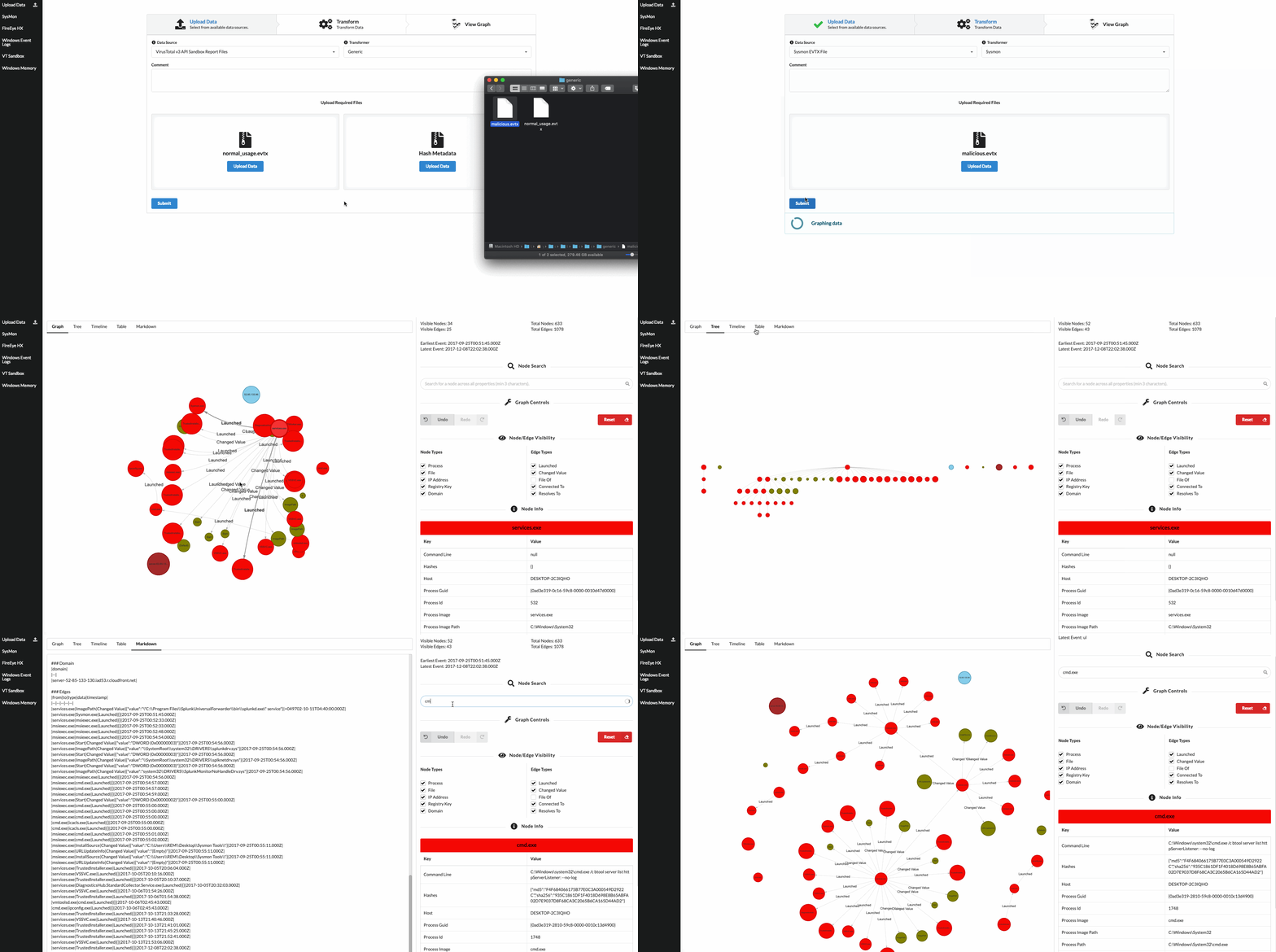
Beagle's docker image comes with a web interface that wraps around the process of both transforming data into graphs, as well as using them to investigate data.
The upload form wraps around the graph creation process, and automatically uses NetworkX as the backend. Depending on the parameters required by the data source, the form will either prompt for a file upload, or text input. For example:
- VT API Sandbox Report asks for the hash to graph.
- FireEye HX requires the HX triage.
Any graph created is stored locally in the folder defined under the dir key from the storage section in the configuration. This can be modified by setting the BEAGLE__STORAGE__DIR environment variable.
Optionally, a comment can be added to any graph to better help describe it.
Each data source will automatically extract metadata from the provided parameter. The metadata and comment are visible later on when viewing the existing graphs of the datasource.
Clicking on a datasource on the sidebar renders a table of all parsed graphs for that datasource.
Viewing a graph in Beagle provides a web interface that allows analysts to quickly pivot around an incident.
The interface is split into two main parts, the left part which contains various perspectives of the graph (Graph, Tree, Table, etc), and the right part which allows you to filter nodes and edges by type, search for nodes, and expand a node's properties. It also allows you to undo and redo operations you perform on the graph.
Any element in the graph that has a divider above it is collapsible:
Nodes in the graph display the first 15 characters of a specific field. For example, for a process node, this will be the process name.
Edges simply show the edge type.
A single click on a node or edge will focus that node and display its information in the "Node Info" panel on the right sidebar.
A double click on a node will pull in any neighbouring nodes. A neighbouring node is any node connected to the clicked-on node by an edge. If there are no neighbors to be pulled in, no change will be seen in the graph.
- This is regardless of direction. That means that a parent process or a child process could be pulled in when double clicking on a node.
- Beagle will only pull in 25 nodes at a time.
A long single click on a node will hide it from the graph, as well as any edges that depend on it.
Right clicking on a node exposes a context menu that allows you to run graph mutators. Mutators are functions which take the graph state, and return a new state.
Two extremely useful mutators are:
- Backtracking a node: Find the sequence of nodes and edges that led to the creation of this node.
- Backtracking a process node will show its process tree.
- Expanding all descendants: From the current node, show every node that has this node as an ancestor.
- Expanding a process node will show every child process node it spawned, any file it may have touched, and pretty much every activity that happened as a result of this node.
Backtracking a node is extremely useful and is similar to doing a root cause infection in log files.
Expanding a node's descendants allows you to immediately view everything that happened because of this node. This action reveals the subgraph rooted at the selected node.
Sometimes, a Node or Edge might not be relevant to the current incident, you can toggle edge and node types on and off. As soon as the type is toggled, the nodes or edges of that type are removed from the visible graph.
Toggling a node type off prevents that node type to be used when using mutators, or when pulling in neighbours.
Any action in the graph is immediately reversible! Using the undo/redo buttons you can revert any action you perform. The reset button sets the graph state to when it loaded, saving you a refresh.
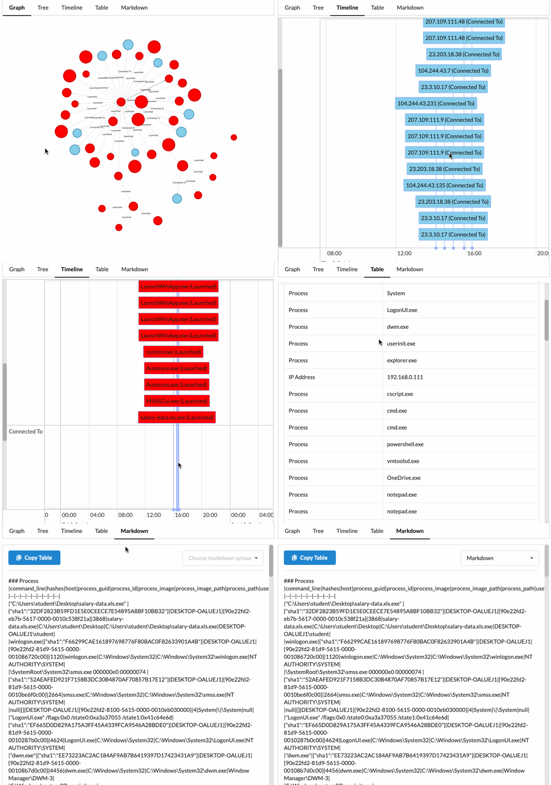
As you change the graph's current state using the above action, you might also want to view the current set of visible node and edges in a different perspective. The tabs at the top of the graph screen allow you to transform the data into a variety of views:
- Graph (Default perspective)
- Tree
- Table
- Timeline
- Markdown
Each of the perspectives supports focusing on nodes by clicking on them.
The graph generation process can be performed programmatically using the python library. The graph generation process is made up of three steps:
DataSourceclasses parse and yield events one by one.Transformerclasses take those inputs and transform them into variousNodeclasses such asProcess.Backendclasses take the array of nodes, place them into a graph structure, and send them to a desired location.
The Python package can be installed via pip:
pip install pybeagleCreating a graph requires chaining these together. This can be done for you using the to_graph() function.
from beagle.datasources import HXTriage

# By default, using the to_graph() class uses NetworkX and the first transformer.
G = HXTriage('test.mans').to_graph()
<networkx.classes.multidigraph.MultiDiGraph at 0x12700ee10>
It can also be done explicitly at each step. Using the functional calls, you can also define which Backend you wish to use for example, to send data to DGraph
from beagle.datasources import HXTriage
from beagle.backends import DGraph
from beagle.transformers import FireEyeHXTransformer

# The data will be sent to the DGraph instance configured in the
# configuration file
backend = HXTriage('test.mans').to_graph(backend=DGraph)

# Can also specify the transformer
backend = HXTriage('test.mans').to_transformer(transformer=FireEyeHXTransformer).to_graph(backend=DGraph)
When calling the to_graph or to_transformer methods, you can pass in any arguments to those classes:
from beagle.datasources import HXTriage
from beagle.backends import Graphistry

# Send the graphistry, anonymize the data first, and return the URL
graphistry_url = HXTriage('test.mans').to_graph(backend=Graphistry, anonymize=True, render=False)
You can also manually invoke each step in the above process, accessing the intermediary outputs
>>> from beagle.backends import NetworkX
>>> from beagle.datasources import HXTriage
>>> from beagle.transformers import FireEyeHXTransformer

>>> datasource = HXTriage("test.mans")
>>> transformer = FireEyeHXTransformer(datasource=datasource)
>>> nodes = transformer.run()
>>> backend = NetworkX(nodes=nodes)
>>> G = backend.graph()
If you want to manually call each step, you will need to ensure that the Transformer class instance is compatible with the output of the provided DataSource class.
- All Backends are compatible with all Transformers.
Each data source defines the list of transformers it is compatible with, and this can be accessed via the .transformers attribute:
>>> from beagle.datasources import HXTriage
>>> HXTriage.transformers
[beagle.transformers.fireeye_hx_transformer.FireEyeHXTransformer]By default, edges are not condensed, that means that if a process node u writes to a file node v 5000 times, you will have 5000 edges between those nodes. Sometimes, especially when trying to visualize the data, this may overwhelm an analyst.
You can condense all 5000 edges into a single edge for that type of action (wrote in this case), by passing the backend class the consolidate_edges=True parameter, for example:
SysmonEVTX("data/sysmon/autoruns-sysmon.evtx").to_graph(NetworkX, consolidate_edges=False)
# Graph contains 826 nodes and 2469 edges.

SysmonEVTX("data/sysmon/autoruns-sysmon.evtx").to_graph(NetworkX, consolidate_edges=True)
# Graph contains 826 nodes and 1396 edges
By default, the web interface will consolidate the edges.


