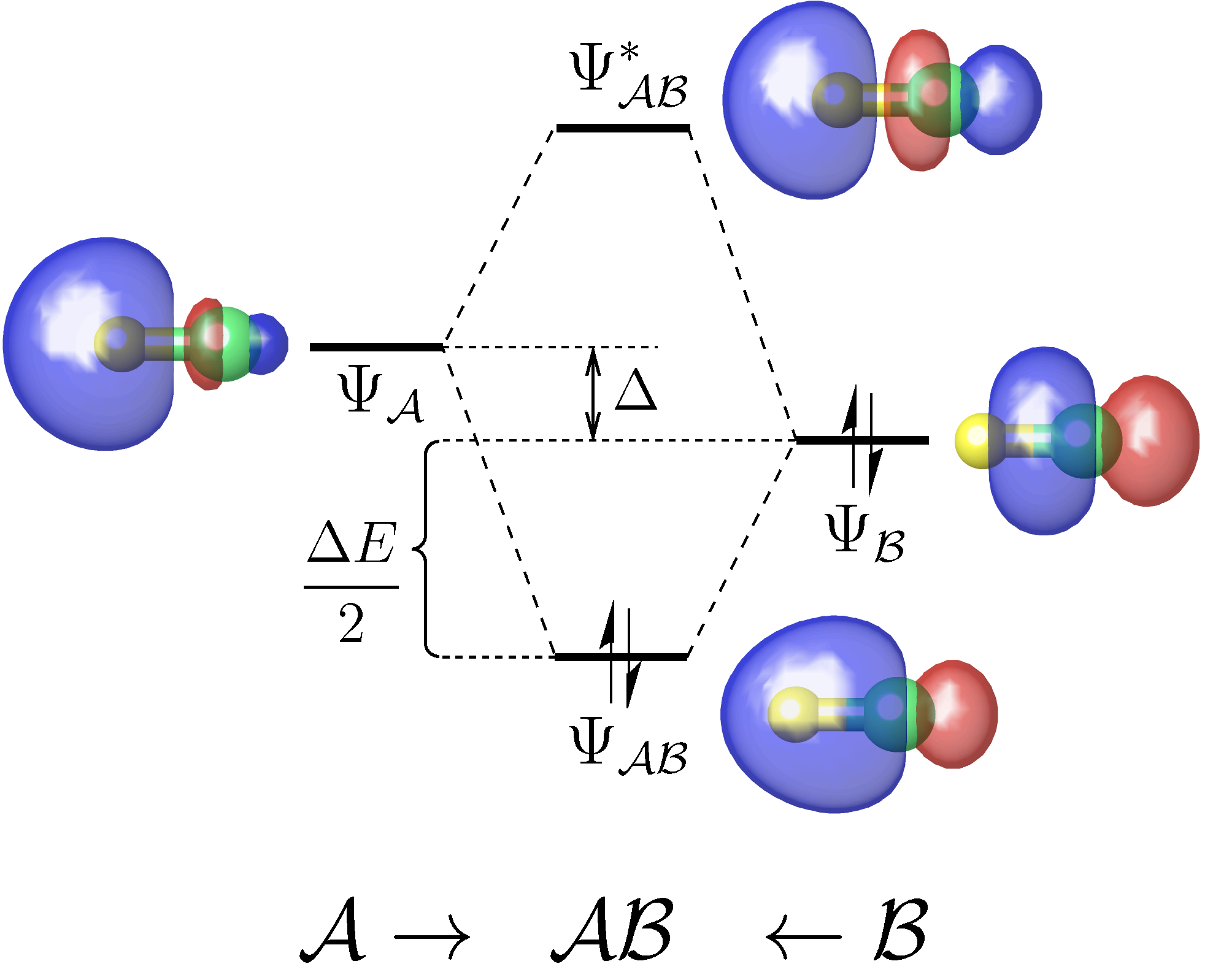
A useful tool for analyzing the chemical interactions between any two fragments of a molecule on the basis of a standard DFT or Hartree-Fock calculation.
Download link for the latest v1.1 version: https://github.com/yangwangmadrid/mbfo/releases/download/v1.1/mbfo_v1.1_release.zip
If you have used the mbfo program in your research papers or presentations, it is obligatory to cite the following paper:
- Yang Wang. Maximum bonding fragment orbitals for deciphering complex chemical interactions. Phys. Chem. Chem. Phys. 2018, 20, 13792-13809. DOI:10.1039/C8CP01808A
- Yang Wang. The mbfo program. 2023. https://github.com/yangwangmadrid/mbfo.
The Author of the mbfo program is Yang Wang ([email protected]; orcid.org/0000-0003-2540-2199). The mbfo program is released under GNU General Public License v3 (GPLv3).
The mbfo program is provided as it is, with no warranties. The Author shall not be liable for any use derived from it. Feedbacks and bug reports are always welcome ([email protected]). However, it is kindly reminded that the Author does not take on the responsibility of providing technical support.
- python >= 3.6
- numpy >= 1.18.0
- scipy >= 1.5.1
- matplotlib >= 3.5.1
- Place the folder of the mbfo package to any location as you like, which is referred to as the source directory hereafter.
- In the source directory, copy the template file "mbfo_v*_template.sh" to "mbfo" and make the latter executable in command line:
cp mbfo_v*_template.sh mbfo
chmod a+x mbfo
Then, open file "mbfo" with a text editor and set the MBFO_DIR variable as the path of the source directory.
- Add the source directory to the global environment variable
PATHin e.g., ".bash_profile" or ".bashrc" under your HOME directory. To this end, the following line (as an example) can be added to ~/.bash_profile:
export PATH=$PATH:${HOME}/softwares/mbfo_v1.0_release
Now, type the following command in terminal window to take effect immediately:
source ~/.bash_profile
- Type
mbfoin your terminal window. If the program is installed correctly, you shall see the following output:
mbfo version x.x (*** 2023)
  -- A program for Maximum Bonding Fragment Orbtal (MBFO) analysis
Written by Yang WANG [[email protected]]
Copyright 2023 Yang Wang

Usage: python mbfo.py <input-file>
- In the Gaussian input file (e.g., abc.gjf), add in the route section the
keywords
fchk=All Pop=NBO6Read, and at the end of the file add$NBO NOBOND AONAO=W $END. In this way, the checkpoint file "Test.FChk" and the NBO matrix file "abc.33" will be generated. Then, rename "Test.FChk" to "abc.fchk". The Gaussian output file should have the extension name of ".out" (If necessary, "abc.log" ought to be renamed as "abc.out").
NOTES:
- It is strongly recommended to use the NBO program later than version 5.0. The free version of NBO 3.1 implemented in Gaussian package would be problematic and give unreliable results.
- Do not use
fchk=Allto generate the checkpoint file if there are two such jobs running at the same working directory at the same time. Otherwise, the two jobs will write the same "Test.FChk" file. Instead, add the%chk=abc.chkline to obtain the checkpoint file "abc.chk". Then, use Gaussian's formchk utility to convert "abc.chk" to "abc.fchk".
- Make sure that at least the following two files, as the inputs for mbfo, are in the same working directory:
- abc.fchk
- abc.33
-
Change to the working directory and prepare the input file for mbfo (vide infra), e.g., "abc.inp". The keywords and options in the input file will be explained below in order to conduct a user-specified MBFO analysis.
-
Simply execute the following command:
mbfo abc.inp > abc.mbfo
As you see, you will find the MBFO analysis results in file "abc.mbfo".
Taking
First, we carry out a DFT single-point calculation, based on the optimized geometry, to obtain the two files, PtCl4-2.fchk and PtCl4-2.33, as required by the mbfo program. The Gaussian's input file (PtCl4-2.gjf) for producing the above two files is as follows:
# PBEPBE/Def2TZVPP fchk=All Pop=NBO6Read NOSYMM

From PtCl4-2_opt.out

-2 1
    78   -1.542120   -1.576087    0.000000
    17    0.818936   -1.576087    0.000000
    17   -1.542120    0.784968   -0.000000
    17   -3.903175   -1.576087    0.000000
    17   -1.542120   -3.937142   -0.000000

$NBO
  NOBOND
  AONAO=W
$END
Next, we prepare a text file named PtCl4-2.inp with the following content:
File =  PtCl4-2        # Key name of the files for the calculated system
Frag = 1               # Index(es) of the atoms for defining fragment A
WriteOrb = MBFO, MBO   # Write the MBFOs and MBOs to external fchk files
PlotCut = 0.1          # Only plotting MBFOs/MBOs with BO > this threshold
ExportPlot = TRUE      # Export the orbital diagram to a *_diagram.pdf file
NOTE:
i) The letters in mbfo's input file are case-insensitive.
ii) All text following the '#' sign is commentary.
iii) Indices of atoms for Frag can be defined in a more compact way following the MATLAB colon syntax and the order does not matter, for example:
Frag = 10, 3:5 9 8/1
This example means that seven atoms, 1, 3, 4, 5, 8, 9 and 10, are defined as fragment A while the rest of atoms are defined as fragment B.
Then, we run mbfo using the following command under the working directory:
mbfo PtCl4-2.inp > PtCl4-2.mbfo
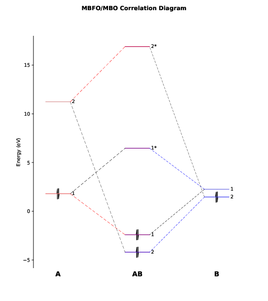
We will see a graphic window pop up showing the orbital correlation diagram, as follows.
This diagram has also been exported to the file PtCl4-2_diagram.pdf.
As we can see, there are only two major bonding interactions between PlotCut in PtCl4-2.inp). In the output file PtCl4-2.mbfo, we can find the BO values of these two major bonding interactions, being 0.997 and 0.785:
No.      BO  Occ(A)  Occ(B)     E(A)     E(B)    E(AB)   E*(AB)    Eint
------------------------------------------------------------------------
  1 0.99728 1.05212 0.94788     1.79     2.26    -2.41     6.46   -8.41
  2 0.78525 0.53659 1.46341    11.24     1.46    -4.20    16.90  -11.32
... ...
TOT 1.95144                                                      -21.77
Both BO values are close to 1 and the total BO between
Hybridization of MBFOs (alpha+beta spin):
                 MBFO(A)                         MBFO(B)
------------------------------------------------------------------------
No.     s    p    d    f    g    h      s    p    d    f    g    h
------------------------------------------------------------------------
  1  0.00 0.00 1.00 0.00 0.00 0.00   0.08 0.91 0.01 0.00 0.00 0.00
  2  0.93 0.00 0.07 0.00 0.00 0.00   0.21 0.79 0.00 0.00 0.00 0.00
... ...
We see that the first MBFO of
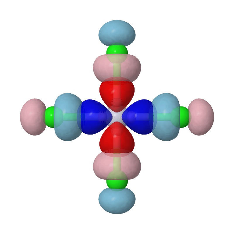
To further to confirm the above analysis, we shall like to visualize these two leading pairs of MBFOs to see their shapes and how they overlap with each other. To this end, we need to generate from the PtCl4-2_MBFO.fchk file the cube file of these MBFOs by using Gaussian's cubegen utility:
cubegen 0 mo=1 PtCl4-2_MBFO.fchk PtCl4-2_MBFO-A1.cube -3 h
cubegen 0 mo=23 PtCl4-2_MBFO.fchk PtCl4-2_MBFO-B1.cube -3 h
cubegen 0 mo=2 PtCl4-2_MBFO.fchk PtCl4-2_MBFO-A2.cube -3 h
cubegen 0 mo=24 PtCl4-2_MBFO.fchk PtCl4-2_MBFO-B2.cube -3 h
Open the cube files PtCl4-2_MBFO-A1.cube and PtCl4-2_MBFO-B1.cube with JMol, we can visualize the overlap between the first pair of MBFOs using the following script in JMol's console:
zap
set frank off
background white
load PtCl4-2_MBFO-A1.cube
isosurface A cutoff 0.05 sign red blue PtCl4-2_MBFO-A1.cube translucent 0.3
isosurface B cutoff 0.05 sign pink skyblue PtCl4-2_MBFO-B1.cube translucent 0.3
As we can see, the most important interaction is basically the chemical bonding between Pt's d(x2-y2) orbital and Cls' p orbitals. The second pair of MBFOs can be visualized by JMol in a similar way:
zap
set frank off
background white
load PtCl4-2_MBFO-A2.cube
isosurface A cutoff 0.05 sign red blue PtCl4-2_MBFO-A2.cube translucent 0.3
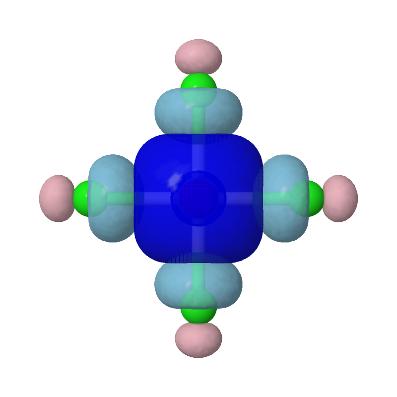
isosurface B cutoff 0.05 sign pink skyblue PtCl4-2_MBFO-B2.cube translucent 0.3
Evidently, the second most important bonding is practically between Pt's s orbital and each of the Cls' sp4 hybridized orbitals.
-
Plot:boolWhether or not plot the orbital correltion diagram for MBFOs/MBOs Default: TRUE -
PlotCut:a positive_valueora negative_valueIn the orbital correltion diagram, only draw MBFOs/MBOs with a bond order (or an orbital interaction energy) more significant than the cutoff value. Positive and negative cutoff refer, respectively, to bond order and interaction energy in kcal/mol. Default: 0.01 -
LabelPlot:TRUEorFALSEWhether or not show the labeling of MBFO/MBO levels in the orbital correltion diagram Default: TRUE -
PrintPop:boolWhether or not print population analysis based on the Mulliken scheme and on the natural atomic orbitals Default: FALSE -
WriteOrb:MBFOand/orMBOand/orNAOand/orAOWrite the corresponding orbtials to external fchk files Default: None


